In the previous chapter we ran the simplex method through dictionaries: rewrite, pivot, repeat. That view is good for intuition. In this chapter we work out the linear algebra behind it. Every dictionary you wrote is a statement about matrices: choosing a basis means selecting an invertible submatrix , pivoting means changing that submatrix, and the objective row of a dictionary is a vector of reduced costs computed from . Making this precise explains why the method works, and it is how simplex is implemented in software, where solvers manipulate basis matrices rather than rewrite equations.
We proceed in two steps. Section 8.1 shows how partitioning variables into basic and nonbasic sets turns into a formula for basic solutions. Section 8.2 then rewrites the objective from the perspective of a basis, giving an algebraic certificate of optimality.
Learning Outcomes
Explore how a system of equations can be rewritten via partitioning the variables
See how we can also partition the matrix and rewrite the equation in a new format that solves for basic variables
Familiarize with matrix notation
Define terminology of a basic solution and a basic feasible solution
We will now explore ways to represent solutions to this linear system of equations. This is meant to give the theoretical backbone of the simplex algorithm.
We consider a linear system
where , , and . Explicitly,
We assume:
, i.e., the rows of are linearly independent (full row rank);
, so the system is not overdetermined.
If lacked full row rank, some equations would be redundant and removable without changing the solution set. When , the system is typically overdetermined and inconsistent; if consistent, it can be reduced to via row operations.
Under these assumptions, represents a system of independent equations in unknowns with a feasible (possibly infinite) solution space.
A small bakery produces two products: loaves of bread (denoted by ) and cakes (denoted by ). Each loaf of bread contributes $2 in profit, while each cake contributes $3 in profit. The bakery must operate under the following daily constraints:
Oven Time: The total number of bread loaves and cakes baked each day cannot exceed 9, due to limited oven time. This gives the constraint:
Flour Supply: Bread uses more flour than cake. Each loaf uses 2 units of flour and each cake uses 1 unit. The bakery has a maximum of 16 units of flour available each day, leading to:
Sugar Supply: Cakes use more sugar than bread. Each loaf uses 1 unit of sugar and each cake uses 2 units. The daily sugar supply is limited to 14 units, so:
Non-negativity: The bakery cannot produce a negative number of items, so:
Model:
The bakery wants to determine how many loaves of bread () and cakes () to produce each day in order to maximize total profit. The resulting linear program is:
We begin by adding slack variables to convert the inequalities to equalities:
It will be useful to also understand standard form from the matrix perspective.
In matrix-vector notation, define:
The standard form linear program is then:
We extract submatrices of by selecting columns corresponding to specific variable sets. For a set , we let denote the submatrix of corresponding to the columns in .
This implies:
So,
In solving the system in the context of linear programming, we introduce the concept of partitioning the variables. This approach is essential in the Simplex Method for identifying and analyzing basic solutions.
Definition 8.1: Basis
Given a matrix of full row rank , a basis is an index set of of the columns such that the corresponding columns of the matrix are linearly independent. We then form the submatrix that contains only those columns of .
The remaining columns are referred to as the nonbasic columns, which form the matrix .
Given a basis and the nonbasic set , this partitions the variable vector into two sets:
where:
consists of the basic variables, associated with the basis matrix ,
consists of the nonbasic variables, associated with the nonbasic matrix .
Rewriting the system in terms of these partitions gives:
| (8.1) |
If the basis matrix is invertible, we can express in terms of :
| (8.2) |
Definition 8.2: Basic solution and Basic Feasible Solution (BFS)
A basic solution is obtained by setting , yielding:
| (8.3) |
A basic feasible solution (BFS) is a basic solution that satisfies the nonnegativity constraint , ensuring that all basic variables are nonnegative.
Consider the following system:
Here, the matrix and the variable vector are:
Selecting as the basis, the corresponding submatrix is:
If is invertible, we compute:
Setting (i.e., ), we solve for :
Since , this is a basic feasible solution.
Consider a linear program in inequality form:
We introduce slack variables to convert inequalities into equalities:
The augmented system has:
Choosing the slack variables as the basis (), the basis matrix is:
Since is the identity matrix, its inverse is itself, and we obtain:
Since , this is a basic feasible solution.
To convert the given problem into standard form, we introduce slack variables to convert the inequalities into equalities.
Now the system is in standard form:
A basis consists of any two linearly independent columns from . We select three different bases:
Basis 1: (Feasible) The basis matrix is:
Computing :
Computing the basic solution:
Since contains no negative values, this basis indeed yields a feasible solution.
Basis 2: (Infeasible) The basis matrix (the columns of and ) is:
Computing :
Computing the basic solution:
Since , this basis is infeasible. The corresponding point is , which violates the constraint .
Basis 3: (Feasible) The basis matrix is:
Since this is the identity matrix, its inverse is itself. Thus, the basic solution is:
Since all basic variables are nonnegative, this is a feasible solution.
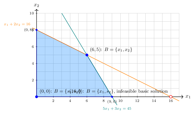
Figure 8.1 shows where these three basic solutions sit relative to the feasible region.
Learning Outcomes
Define reduced costs at a basic feasible solution
Establish optimality conditions via the reduced costs
The objective function of the linear program is given by:
Substituting the partitioned variables and ,
Expressing in terms of , using the basic solution , we rewrite the objective function as:
| (8.4) |
Expanding and regrouping terms:
| (8.5) |
Definition 8.3: Reduced Costs
The term represents the reduced costs.
This is explained as the objective rewritten from the viewpoint of a basic feasible solution. In particular, these are the coefficients on the non-basic variables.
The system is rewritten as the dictionary form at basis as in the following definition.
Definition 8.4: Revised Simplex Dictionary at basis
The revised simplex dictionary at a basis is
| (8.6) |
Here is an example: the same linear program written first at the slack basis and then at the basis .
Theorem 8.5: Optimality Condition in Simplex Method
Given a linear program in standard form:
let be a basis corresponding to a basic feasible solution , with nonbasic variables .
If all reduced costs satisfy:
then the current basic feasible solution is optimal.
Proof. Let .
If all reduced costs are nonpositive, i.e.,
then for any feasible choice of , we have
where the last line follows since and .
Thus, is an optimal solution! □
A note on sign conventions. The three treatments of the simplex method in this book state the same optimality test in three ways. In the dictionary form of Chapter 7, we improve the solution by increasing a nonbasic variable with a positive coefficient in the objective row, and we stop when there is none. The theorem above says the same thing in matrix language: those coefficients are the reduced costs , and the solution is optimal once they are all . In the tableau form of Chapter 9, the objective is stored as the equation , which flips the signs of these coefficients, so there you look for negative -row entries and stop when every entry is nonnegative. All three are the same test.
Example 8.6: Verifying Optimality Using Reduced Costs
We aim to verify that the basic feasible solutions and are optimal for the following linear program:
Solution
Checking Optimality of
Step 1 — Identify the Basis. At the point , we see that . Thus, we can choose and , so:
The nonbasic variables are , so:
Step 2 — Compute .
Thus, the system can be written as
that is
(8.10) or equivalently
(8.11)
Step 3 — Compute Reduced Costs.
Computing:
The reduced cost on is positive (), so is not optimal: increasing improves the objective.
Verifying Optimality of
Step 1 — Identify the Basis.
At the point we have and , so the basic variables are and . We choose , so:
The nonbasic variables are , so:
Step 2 — Compute .
As a check, , matching : a basic feasible solution.
Step 3 — Compute Reduced Costs.
Since both reduced costs are negative, this confirms that is an optimal solution.
Conclusion
is not necessarily optimal because it has a positive reduced cost.
is optimal because all reduced costs are nonpositive.
The reduced-cost computation we just carried out is the algebraic version of a picture worth revisiting: every vertex of the feasible region has its own dictionary, and the signs of its reduced costs say whether a better neighbor exists. See Figure 7.4 in Section 7.3 for that vertex-by-vertex view.
Resources
Desmos: Interactive plot of an LP from different BFS perspectives (backup interactive plot).
Exercise 8.7: Basis matrix and basic solution
Consider the system from Example 1,
and take the basis .
[§8.1, Example 1]
Exercise 8.8: A basic solution that is not feasible
For the same system as Exercise 8.7, take the basis . Compute , , and the basic solution, and explain why this basis gives a basic solution that is not feasible.
[§8.1, Example 1]
Exercise 8.9: A fourth basis for the three-bases example
In Section 8.1.3 we evaluated the bases , , and of the system
Now evaluate the basis : compute , , and the basic solution, and decide whether it is feasible. Which point does this basis correspond to?
[§8.1.3]
Exercise 8.10: Reduced costs at two bases
Consider the bakery linear program of Section 8.1 in standard form,
with variables ordered . For each of the bases
compute , the basic solution , the objective value , and the reduced costs . Use the optimality condition to decide whether each basis is optimal.
Exercise 8.11: Which bases are feasible?
For the system
there are ways to choose two columns.
Exercise 8.12: Rebuilding a dictionary from the formula
Section 8.2 displays the linear program
together with its dictionary at the basis . Using the revised simplex dictionary formula (8.6), compute , , , and the reduced costs, and confirm that the formula reproduces the displayed dictionary
[§8.2]
Exercise 8.13: Reduced costs of basic variables
The reduced-cost vector of the nonbasic variables is . Apply the same formula to the basic columns: show that
so every basic variable has reduced cost exactly zero. Explain what this says about the dictionary at basis : why can a basic variable never appear in the objective row?
[§8.2]
Exercise 8.14: Reduced-cost signs and the entering rule
In the dictionary form of Chapter 7, the entering variable is a nonbasic variable with a positive coefficient in the objective row, while the optimality theorem of this chapter stops when all reduced costs are .
[§8.2, sign-convention paragraph; §8.2]
Exercise 8.15: Strictly negative reduced costs imply a unique optimum
Let be a basis of an LP in standard form whose basic solution is feasible, and suppose every reduced cost is strictly negative:
Prove that is the unique optimal solution of the LP. (This is an argument, not a computation. Suggested route: take any feasible , write , and consider the two cases and .)
[§8.2, Optimality Condition theorem]
Solution
(Exercise 8.7) The columns of and give
The basic solution is
so . Both basic variables are nonnegative, so this is a basic feasible solution.
Solution
(Exercise 8.10) Basis . Ordering the basic variables ,
so , , : a basic feasible solution with objective value . The nonbasic variables are and , and the reduced costs work out to
The reduced cost of is , so is not optimal; this matches the second dictionary of Chapter 7, .
Basis . Here
a basic feasible solution with value . The nonbasic variables are and , with reduced costs
so is optimal, matching the final dictionary .
Solution
(Exercise 8.15) Write and . Every feasible satisfies , so and, exactly as in the optimality theorem,
Take any feasible .
Case 1: . Then some component with , and since every entry of is strictly negative, . Hence , so is not optimal.
Case 2: . Then , and since is invertible this forces , i.e., , contradicting .
Therefore every feasible point other than has objective value strictly less than : the solution is optimal and no other optimal solution exists.