7 Simplex Method

Contents | ‹ Previous | Next › | Download EPUB | PDF

Chapter 7
Simplex Method

Learning Outcomes

Convert linear programs to standard form
Reformulate linear programs from the perspective of different bases
Define basic solutions and basic feasible solutions
Describe optimality condition from the perspective of a reformulation
Develop the Simplex Method that pivots through basic feasible solutions

Picture hiking to the highest point of a fenced field on a moonless night. Your flashlight shows only the ground at your feet: the corner you are standing on and the fence lines leading away from it. A sensible strategy suggests itself: shine the light along each fence line; if one leads uphill, follow it to the next corner and look again; if none does, stop. The remarkable fact of this chapter is that for linear programs this nearsighted strategy is guaranteed to end at the highest point of the entire field. The algebra of “shining the flashlight” is a reformulation of the linear program called a dictionary.

In this section, we will develop the Simplex Method. This algorithm has been lauded as one of the most important algorithms of the 20th century. It will iteratively find better vertex solutions to a linear program until it can prove optimality.

To implement the simplex algorithm, we must first discuss a Standard Form with which to represent linear programs. After, we will discuss structure of linear programs in this form using matrix notation and demonstrate how a linear program can be transformed to new representations. These new representations will be the backbone of the simplex algorithm. We will pivot between vertices, and each vertex will have a new representation of the linear program that will help us understand how to choose a new vertex to move to.

The whole algorithm runs very fast in practice. Here, we will teach you a basic version of the algorithm, but note that state-of-the-art solvers will employ a number of tricks to make this process very fast. Linear programs can be solved with millions of variables!

7.1 Standard Form

To solve a linear program using methods such as the simplex algorithm, the problem must first be converted to a standard form. This ensures the problem adheres to a uniform structure, making it easier to analyze and solve algorithmically.

A linear program is in standard form if it satisfies all of the following:

The objective is a maximization.
All constraints are equalities (i.e., of the form $=$ ).
All variables are bounded below by zero (i.e., $x_{i} \geq 0$ ).

Definition 7.1: Standard Form

A linear program is in standard form if it is written as

\begin{array}{l} \max & c^{⊤} x \\ s . t . & A x = b \\ x \geq 0 . \end{array}

7.1.1 Converting to Standard Form

We now describe how to handle each of these aspects step-by-step, including common subcases and examples.

1. Objective: Convert Minimization to Maximization

If the linear program is given as a minimization, we convert it into a maximization by multiplying the objective function by $- 1$ . This transformation does not affect the feasible region, and the maximizer of the new function will be the minimizer of the original.

Example 7.2: Convert Min to Max

Consider the following objective:

\min 3 x_{1} + 4 x_{2} .

To convert this to a maximization, we multiply the entire expression by $- 1$ :

\max (- 3 x_{1} - 4 x_{2}) .

Now the problem can be treated using standard methods that assume a maximization objective.

2. Constraints: Convert Inequalities to Equalities

All inequality constraints must be transformed into equalities using slack or surplus variables, which represent the difference between the left- and right-hand sides of the constraint.

Convert $\leq$ to $=$ using a slack variable.

A slack variable is added to "fill the gap" in a $\leq$ constraint and must be nonnegative.

Example 7.3: Slack Variable for $\leq$

Suppose we have the constraint:

$x_{1} + 2 x_{2} \leq 5 .$

We introduce a new variable $s_{1} \geq 0$ , called a slack variable, and rewrite the constraint as:

$x_{1} + 2 x_{2} + s_{1} = 5 .$

Here, $s_{1}$ represents the unused portion of the right-hand side (i.e., how far the left-hand side is from 5).

Convert $\geq$ to $=$ using a surplus variable.

A surplus variable is subtracted from the left-hand side of a $\geq$ constraint to convert it into an equality. This variable also must be nonnegative.

Example 7.4: Surplus Variable for $\geq$

Consider the constraint:

$x_{1} - x_{2} \geq 3 .$

We introduce a new variable $s_{2} \geq 0$ , called a surplus variable, and rewrite the constraint as:

$x_{1} - x_{2} - s_{2} = 3 .$

In this case, $s_{2}$ accounts for the extra amount by which the left-hand side exceeds 3.

3. Variable Bounds: Ensure All Variables Are Nonnegative

The standard form requires all variables to satisfy $x_{i} \geq 0$ . If any variable is unbounded below or is restricted in another way, we perform a variable substitution to enforce this condition.

Convert $x_{i} \leq 0$ to $x_{i}^{'} \geq 0$ by renaming and negating.

If a variable is constrained to be nonpositive, we can define a new nonnegative variable as its negation.

Example 7.5: Rename and Negate for $\leq 0$

Suppose $x_{3} \leq 0$ . Define $x_{3}^{'} = - x_{3}$ , which implies $x_{3}^{'} \geq 0$ . Then substitute:

$x_{3} = - x_{3}^{'}, where x_{3}^{'} \geq 0 .$

This transformation allows us to enforce nonnegativity in the standard form.

Convert unrestricted variables into the difference of two nonnegative variables.

If a variable is unrestricted in sign (i.e., it can be positive or negative), we express it as the difference of two new nonnegative variables.

Example 7.6: Unrestricted Variable to Two Variables

Suppose $x_{4}$ is unrestricted. We define:

$x_{4} = x_{4}^{+} - x_{4}^{-}, with x_{4}^{+}, x_{4}^{-} \geq 0 .$

Here, $x_{4}^{+}$ captures the positive part and $x_{4}^{-}$ captures the negative part. At most one of them will be nonzero in a basic feasible solution.

After performing these transformations, the resulting linear program will be in standard form and ready for solution via the simplex method or other standard techniques.

Example 7.7: Complete Conversion to Standard Form

Consider the following linear program:

\begin{aligned} \min & 2 x_{1} - 3 x_{2} + x_{3} \\ s.t. & x_{1} - x_{2} \leq 4, \\ 2 x_{1} + x_{3} = 7, \\ x_{2} - x_{3} \geq 2, \\ x_{1} is unrestricted, x_{2} \geq 0, x_{3} is unrestricted . \end{aligned}

We will now convert this problem into standard form.

Step 1: Convert the objective to maximization.

Since the problem is a minimization, we multiply the objective by $- 1$ :

\max (- 2 x_{1} + 3 x_{2} - x_{3}) .

Step 2: Replace unrestricted variables.

Both $x_{1}$ and $x_{3}$ are unrestricted. We express them as the difference of two nonnegative variables:

x_{1} = x_{1}^{+} - x_{1}^{-}, x_{3} = x_{3}^{+} - x_{3}^{-}, with x_{1}^{+}, x_{1}^{-}, x_{3}^{+}, x_{3}^{-} \geq 0 .

Substitute these into the objective and constraints.

New objective:

\max [- 2 (x_{1}^{+} - x_{1}^{-}) + 3 x_{2} - (x_{3}^{+} - x_{3}^{-})] = \max (- 2 x_{1}^{+} + 2 x_{1}^{-} + 3 x_{2} - x_{3}^{+} + x_{3}^{-}) .

New constraints:

\begin{array}{l} (x_{1}^{+} - x_{1}^{-}) - x_{2} & \leq 4 & (original 1st constraint) \\ 2 (x_{1}^{+} - x_{1}^{-}) + (x_{3}^{+} - x_{3}^{-}) & = 7 & (original 2nd constraint) \\ x_{2} - (x_{3}^{+} - x_{3}^{-}) & \geq 2 & (original 3rd constraint) \end{array}

Step 3: Convert inequalities to equalities.

Add a slack variable $s_{1} \geq 0$ to the first constraint:

$x_{1}^{+} - x_{1}^{-} - x_{2} + s_{1} = 4$

The second constraint is already an equality:

2 x_{1}^{+} - 2 x_{1}^{-} + x_{3}^{+} - x_{3}^{-} = 7

Subtract a surplus variable $s_{2} \geq 0$ from the third constraint:

$x_{2} - x_{3}^{+} + x_{3}^{-} - s_{2} = 2$

Final standard form:

\begin{aligned} \max & - 2 x_{1}^{+} + 2 x_{1}^{-} + 3 x_{2} - x_{3}^{+} + x_{3}^{-} \\ s.t. & x_{1}^{+} - x_{1}^{-} - x_{2} + s_{1} = 4 \\ 2 x_{1}^{+} - 2 x_{1}^{-} + x_{3}^{+} - x_{3}^{-} = 7 \\ x_{2} - x_{3}^{+} + x_{3}^{-} - s_{2} = 2 \\ x_{1}^{+}, x_{1}^{-}, x_{2}, x_{3}^{+}, x_{3}^{-}, s_{1}, s_{2} \geq 0 . \end{aligned}

This is now in standard form: a maximization problem with equality constraints and all variables nonnegative.

Remark. Variable Transformations Preserve Solution Meaning To convert a linear program into standard form, we often introduce new variables:

Slack variables to convert $\leq$ constraints to equalities,
Surplus variables for $\geq$ constraints,
Split unrestricted variables as $x_{j} = x_{j}^{+} - x_{j}^{-}$ ,
Negate variables with $x_{j} \leq 0$ .

These transformations may change the number of variables and the way solutions are expressed, but:

1.: Every feasible solution to the transformed problem corresponds to a feasible solution of the original problem.
2.: Every optimal solution of the transformed problem yields an optimal solution to the original.

Thus, while the form of the solution may look different, the meaning and the value of the solution are preserved.

Two-row diagram: Original LP (min or max, unrestricted variables, inequalities) connected by arrows labeled 'variable transformations / interpret in original space' to Transformed LP in Canonical Form (max, all equalities, variables >= 0); below, Solution to Original LP is connected to Solution to Transformed LP by 'encode to canonical form / map back (e.g., x_j = x_j-plus minus x_j-minus)'. — Figure 7.1: Correspondence between original and canonical form solutions.

Example 7.8: Transformation Preserves Solution Meaning

Consider the following linear program:

\begin{aligned} \min & - x_{1} + 2 x_{2} - 3 x_{3} \\ s.t. & x_{1} - x_{2} + x_{3} \geq 2, \\ x_{2} \leq 0, \\ x_{3} unrestricted . \end{aligned}

Step 1: Convert to maximization.

Multiply the objective by $- 1$ :

\max x_{1} - 2 x_{2} + 3 x_{3} .

Step 2: Convert variables to be nonnegative.

$x_{2} \leq 0$ $⇝$ define $x_{2} = - x_{2}^{'}$ , with $x_{2}^{'} \geq 0$ .
$x_{3}$ unrestricted $⇝$ write $x_{3} = x_{3}^{+} - x_{3}^{-}$ , with $x_{3}^{+}, x_{3}^{-} \geq 0$ .

Substitute into the objective and constraint:

\max x_{1} - 2 (- x_{2}^{'}) + 3 (x_{3}^{+} - x_{3}^{-}) = x_{1} + 2 x_{2}^{'} + 3 x_{3}^{+} - 3 x_{3}^{-} .

Constraint: x_{1} + x_{2}^{'} + x_{3}^{+} - x_{3}^{-} \geq 2 .

Step 3: Convert constraint to equality using a surplus variable.

Introduce surplus variable $s_{1} \geq 0$ :

x_{1} + x_{2}^{'} + x_{3}^{+} - x_{3}^{-} - s_{1} = 2 .

Now the problem is in standard form:

\begin{aligned} \max & x_{1} + 2 x_{2}^{'} + 3 x_{3}^{+} - 3 x_{3}^{-} \\ s.t. & x_{1} + x_{2}^{'} + x_{3}^{+} - x_{3}^{-} - s_{1} = 2, \\ x_{1}, x_{2}^{'}, x_{3}^{+}, x_{3}^{-}, s_{1} \geq 0 . \end{aligned}

Example 7.9: Example Continued

Step 4: Example solution in standard form.

Consider a solution of the canonical form

x_{1} = 1, x_{2}^{'} = 0, x_{3}^{+} = 1, x_{3}^{-} = 0, s_{1} = 0 .

Step 5: Map solution back to original variables.

x_{2} = - x_{2}^{'} = 0, x_{3} = x_{3}^{+} - x_{3}^{-} = 1 .

So the solution to the original problem is:

x_{1} = 1, x_{2} = 0, x_{3} = 1,

and the original objective value is:

- 1 (1) + 2 (0) - 3 (1) = - 4 .

Conclusion: The transformation allowed us to solve the LP using standard techniques, and we were able to directly interpret the solution in the space of the original variables. The solution meaning is preserved.

7.1.2 Basic Feasible Solutions for Standard Form

Consider a linear program in standard form:

\begin{aligned} \max & c^{⊤} x \\ s.t. & A x = b, \\ x \geq 0, \end{aligned}

where $A \in ℝ^{m \times n}$ , $b \in ℝ^{m}$ , and $c \in ℝ^{n}$ .

We assume throughout that:

The matrix $A$ has full row rank, i.e., $rank (A) = m$ ,
The feasible region ${x \in ℝ^{n} : A x = b, x \geq 0}$ is nonempty.

Definition 7.10: Basic Feasible Solution

A vector $x \in ℝ^{n}$ is called a basic feasible solution (BFS) if:

1.: It satisfies all the constraints of the LP (i.e., it is feasible),
2.: It has at most $m$ positive components (i.e., $n - m$ components are set to zero),
3.: These positive components correspond to a set of linearly independent columns of $A$ .

Let $B \subseteq {1, \dots, n}$ be an index set of size $m$ such that the submatrix $A_{B}$ (formed from the columns of $A$ indexed by $B$ ) is nonsingular. Then the corresponding basic solution is given by:

x_{B} = A_{B}^{- 1} b, x_{N} = 0,

where $N = {1, \dots, n} ∖ B$ . If $x_{B} \geq 0$ , the basic solution is feasible, and hence a basic feasible solution.

Basic feasible solutions play a central role in the simplex method, which moves from one BFS to another while improving the objective function value.

Example 7.11: Basic Feasible Solution

Consider the linear program:

\begin{aligned} \max & 3 x_{1} + 2 x_{2} \\ s.t. & x_{1} + x_{2} \leq 4, \\ 2 x_{1} + x_{2} \leq 5, \\ x_{1}, x_{2} \geq 0 . \end{aligned}

We first convert the inequalities to equalities by introducing slack variables $s_{1}$ and $s_{2}$ :

\begin{aligned} x_{1} + x_{2} + s_{1} & = 4, \\ 2 x_{1} + x_{2} + s_{2} & = 5, \\ x_{1}, x_{2}, s_{1}, s_{2} & \geq 0 . \end{aligned}

This system has 4 variables and 2 equality constraints. A basic feasible solution corresponds to choosing any 2 variables (equal to the number of constraints) as basic and solving for them.

Choose $s_{1}$ and $s_{2}$ as the basic variables (so $x_{1} = x_{2} = 0$ ). Substituting into the equations:

\begin{aligned} s_{1} & = 4, \\ s_{2} & = 5 . \end{aligned}

This gives the solution:

(x_{1}, x_{2}, s_{1}, s_{2}) = (0, 0, 4, 5),

which is a basic feasible solution. It is feasible because all variables are nonnegative, and basic because we set two variables (equal to the number of constraints) to nonzero values.

Geometrically, this solution corresponds to the intersection of the two axes (i.e., the origin) in the $(x_{1}, x_{2})$ plane, a corner point of the feasible region.

Learning Checkpoint 7.1.1

In a basic feasible solution (BFS) to a linear program in standard form, how many components of the decision vector $x$ can be nonzero?

[Hint: Relate your answer to the number of linearly independent constraints in the system.]

Proposition 7.1. Vertices and BFS Let $P = {x \in ℝ^{n} : A x = b, x \geq 0}$ be the feasible region of a linear program in standard form, where $A \in ℝ^{m \times n}$ has full row rank $m \leq n$ . Then every vertex of $P$ is a basic feasible solution.

Proof. Let $x^{*} \in P$ be a vertex of the feasible region $P$ . By definition, this means that $x^{*}$ cannot be expressed as a strict convex combination of two distinct points in $P$ . We will show that $x^{*}$ is a basic feasible solution.

Let $I : = {j \in {1, \dots, n} : x_{j}^{*} > 0}$ be the support of $x^{*}$ , and let $A_{I}$ denote the submatrix of $A$ consisting of the columns indexed by $I$ . Since $A x^{*} = b$ , and $x_{j}^{*} = 0$ for $j \notin I$ , the vector $x_{I}^{*} \in ℝ^{| I |}$ satisfies:

A_{I} x_{I}^{*} = b .

If the columns of $A_{I}$ were linearly dependent, then there would exist a nonzero vector $d \in ℝ^{n}$ with support in $I$ such that $A d = 0$ , and for small enough $𝜀 > 0$ , both $x^{*} + 𝜀 d$ and $x^{*} - 𝜀 d$ would remain in $P$ , contradicting the fact that $x^{*}$ is a vertex.

Therefore, the columns of $A_{I}$ must be linearly independent, and since $A$ has rank $m$ , it follows that $| I | \leq m$ . We can now construct a basic solution by selecting any set $B \subseteq {1, \dots, n}$ of indices such that:

$B \supseteq I$ ,
$| B | = m$ ,
The columns $A_{B}$ are linearly independent.

Let $x_{B} = A_{B}^{- 1} b$ , and set $x_{N} = 0$ , where $N = {1, \dots, n} ∖ B$ . Then $x$ is a basic solution. Since $x_{j}^{*} = 0$ for $j \notin I \subseteq B$ , and $x_{j}^{*} > 0$ for $j \in I$ , it follows that $x^{*}$ coincides with this basic solution and is nonnegative; hence it is a basic feasible solution. □

7.2 Canonical Form

For our purposes, it’s not quite enough to have a problem in standard form. We also want to have easy access to a basic feasible solution. Thus, we like to convert linear programs to canonical form.

Definition 7.12: Canonical Form of a Linear Program

A linear program is in canonical form if:

it is in standard form:

$\begin{aligned} \max & c^{⊤} x \\ s.t. & A x = b, \\ x \geq 0, \end{aligned}$
the constraint matrix $A$ contains the identity matrix $I_{m}$ as a submatrix corresponding to some set of basic variables $B \subseteq {1, \dots, n}$ ,
and the right-hand side $b \geq 0$ .

In this case, a basic feasible solution is immediately evident: set the basic variables $x_{B} = b$ , and nonbasic variables to zero.

Example 7.13: Canonical Form from Slack Variables

Consider the linear program:

\begin{aligned} \max & 2 x_{1} + 3 x_{2} \\ s.t. & x_{1} + x_{2} \leq 4, \\ x_{1} + 2 x_{2} \leq 6, \\ x_{1}, x_{2} \geq 0 . \end{aligned}

We convert the $\leq$ constraints to equalities by introducing slack variables $s_{1}$ and $s_{2}$ :

\begin{aligned} x_{1} + x_{2} + s_{1} & = 4, \\ x_{1} + 2 x_{2} + s_{2} & = 6, \\ s_{1}, s_{2} & \geq 0 . \end{aligned}

Now the LP is in standard form with 4 variables $x_{1}, x_{2}, s_{1}, s_{2}$ . The constraint matrix is:

A = [\begin{matrix} 1 & 1 & 1 & 0 \\ 1 & 2 & 0 & 1 \end{matrix}]

The columns corresponding to $s_{1}$ and $s_{2}$ form the identity matrix:

A_{B} = [\begin{matrix} 1 & 0 \\ 0 & 1 \end{matrix}] = I_{2}, and b = [\begin{matrix} 4 \\ 6 \end{matrix}] \geq 0 .

Hence, this LP is now in canonical form. The evident basic feasible solution is:

x_{1} = 0, x_{2} = 0, s_{1} = 4, s_{2} = 6 .

Figure 7.2: When can you use canonical form?

7.2.1 Augmenting system and Phase 1

We can summarize these tricks in the following table.

We end this subsection with a motivating result.

Proposition 7.2. Existence of Canonical Form for Feasible LPs Let $P$ be a linear program in standard form:

\begin{aligned} \max & c^{⊤} x \\ s.t. & A x = b, \\ x \geq 0 . \end{aligned}

If $P$ is feasible (i.e., $\exists x \geq 0$ such that $A x = b$ ), then there exists an equivalent linear program in canonical form, that is, a reformulation where:

$A$ contains the identity matrix $I_{m}$ as a submatrix,
The corresponding basic variables yield a basic feasible solution with $b \geq 0$ ,
The objective function is unchanged in value on feasible solutions.

Idea of Proof. Start from any feasible solution $x \in ℝ^{n}$ with $x \geq 0$ and $A x = b$ . Use the simplex method (or a pivoting method) to move to a basic feasible solution $x^{*}$ . Since $A$ has full rank over the feasible region, the basis matrix $A_{B}$ will be invertible. By reordering variables (i.e., choosing a new basis where $A_{B} = I_{m}$ ), we can express the LP in canonical form.

If no feasible solution exists, then Phase I must be used to find one (or certify infeasibility). □

7.3 Pivoting and the Simplex Algorithm

Learning Outcomes

See an example of the simplex method in action
Formally state the simplex algorithm
See that changing the pivot rule can change the path to the optimal solution

Resources

Video

Youtube! - Simplex Method - Watch 3:40 to 11:40

Interactive Simplex Method

Simplex Dictionary Calculator Using Python + Jupyter

Try it out visually!

Simplex Pivoter in Dictionary Form: pivot this chapter’s bakery example (or your own LP) step by step, with a practice mode that checks your entering and leaving choices.

The Simplex Algorithm jumps among the vertices of the feasible region searching for an optimal point. It does this by moving along the edges of the feasible region in such a way that the objective function is always increased after each move.

To improve the solution, we:

1.: Select an entering variable with a negative reduced cost.
2.: Determine the leaving variable using the minimum ratio test.
3.: Perform a pivot operation to update the basis.

This process continues until no negative reduced costs remain, indicating an optimal solution.

7.3.1 Transforming the LP to Standard Form

We start with the following linear program:

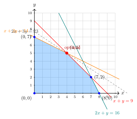
$\begin{aligned} \max & 2 x + 3 y \\ s.t. & x + y & \leq 9, \\ 2 x + y & \leq 16, \\ x + 2 y & \leq 14, \\ x, y \geq 0 . \end{aligned}$

To convert these inequalities to equalities, we introduce slack variables $s_{1}$ , $s_{2}$ , and $s_{3}$ . Specifically, we rewrite each constraint as follows:

\begin{aligned} x + y + s_{1} & = 9, \\ 2 x + y + s_{2} & = 16, \\ x + 2 y + s_{3} & = 14, \end{aligned}

with the additional nonnegativity constraints $s_{1}, s_{2}, s_{3} \geq 0$ .

Hence, the linear program in standard form becomes:

$\begin{aligned} \max & 2 x + 3 y \\ s.t. & x + y + s_{1} = 9, \\ 2 x + y + s_{2} = 16, \\ x + 2 y + s_{3} = 14, \\ x, y, s_{1}, s_{2}, s_{3} \geq 0 . \end{aligned}$

Rewriting the System with ${s_{1}, s_{2}, s_{3}}$ as the Basis

When we say ${s_{1}, s_{2}, s_{3}}$ is the basis, we solve each equation for the corresponding slack variable:

\begin{aligned} s_{1} & = 9 - x - y, \\ s_{2} & = 16 - 2 x - y, \\ s_{3} & = 14 - x - 2 y . \end{aligned}

Our initial non-basic variables are $x$ and $y$ . We will call this representation of the linear program a dictionary.

$\begin{aligned} \max & z = 0 + 2 x + 3 y \\ s.t. & s_{1} = 9 - x - y, \\ s_{2} = 16 - 2 x - y, \\ s_{3} = 14 - x - 2 y, \\ x, y, s_{1}, s_{2}, s_{3} \geq 0 . \end{aligned}$

From here we can read off a basic solution that is
$Basic variables: (s_{1}, s_{2}, s_{3}) = (9, 16, 14),$

$Non-basic variables: (x, y) = (0, 0)$
with
$Objective value: z = 0 .$
Since the basic variables are all non-negative $(\geq 0)$ , we call this a basic feasible solution.

Remark. Reading the Dictionary From the dictionary below, we can read off the corresponding basic solution and the objective value. The basic solution is obtained by:

Setting all nonbasic variables (those on the right-hand side of the equations, i.e., $x$ and $y$ ) equal to zero.
Reading off the values of the basic variables ( $s_{1}, s_{2}, s_{3}$ ) from the right-hand side constants.

The dictionary is said to be feasible if all basic variables have nonnegative values (which is true here). Thus, this corresponds to a basic feasible solution:

x = 0, y = 0, s_{1} = 9, s_{2} = 16, s_{3} = 14, z = 0 .

\begin{aligned} \max & z = 0 + 2 x + 3 y \\ s.t. & s_{1} = 9 - x - y, \\ s_{2} = 16 - 2 x - y, \\ s_{3} = 14 - x - 2 y, \\ x, y, s_{1}, s_{2}, s_{3} \geq 0 . \end{aligned}

7.3.2 Simplex Assuming Feasible Start

In this subsection we assume that the slack basis ${s_{1}, s_{2}, s_{3}}$ gives a feasible starting dictionary; that is, setting the original variables $x, y$ to zero produces nonnegative values for every slack. Under this assumption, the simplex method proceeds by repeatedly choosing an entering variable whose objective-row coefficient is positive, performing the ratio test to decide which basic variable leaves, and pivoting to obtain a new dictionary. The remainder of this section walks through these three steps on the running example above.

We take as our initial basic variables the three slack variables $s_{1}, s_{2}, s_{3}$ . Geometrically, this corresponds to the point $(x, y) = (0, 0)$ . Indeed, if $x = 0$ and $y = 0$ , then from the original constraints

\begin{aligned} x + y + s_{1} & = 9, \\ 2 x + y + s_{2} & = 16, \\ x + 2 y + s_{3} & = 14, \end{aligned}

it follows that

s_{1} = 9, s_{2} = 16, s_{3} = 14 .

All are nonnegative, so $(s_{1}, s_{2}, s_{3})$ is indeed a feasible basis, and $(0, 0, 9, 16, 14)$ is the basic feasible solution (BFS).

Thus, in “basic-variable $=$ constant $-$ (nonbasic terms)” form, our system becomes

{\begin{matrix} s_{1} + x + y = 9, \\ s_{2} + 2 x + y = 16, \\ s_{3} + x + 2 y = 14 . \end{matrix}

Since $s_{1}, s_{2}, s_{3}$ are taken to be the basic variables, the nonbasic variables in this setup are $x$ and $y$ . Setting $x = 0, y = 0$ immediately gives the BFS

(x, y, s_{1}, s_{2}, s_{3}) = (0, 0, 9, 16, 14) .

The Objective Function in this Basis

\max z = 2 x + 3 y .

Value of $z$ at the BFS $(0, 0, 9, 16, 14)$ . At $(x, y) = (0, 0)$ , we see $z = 2 \cdot 0 + 3 \cdot 0 = 0$ , so the initial objective value is $z = 0$ . From here, one would normally proceed with the simplex pivots to drive the objective upwards (since this is a maximization problem). We handle those pivot steps next.

Choosing the Entering Variable

We examine the objective row to determine which nonbasic variable should enter the basis. At this point, the objective is:

$z = 2 x + 3 y .$

The nonbasic variables are $x$ and $y$ .

Both have positive coefficients, which means that increasing either variable (while staying feasible) will increase the objective value $z$ .

To decide between them, we apply a pivot rule, a strategy for selecting among eligible entering variables.

In this example, we use the Steepest Ascent rule: we choose the nonbasic variable with the largest positive coefficient in the objective row.

Between $x$ and $y$ , the coefficient of $y$ is larger ( $3 > 2$ ).

Therefore, we choose $y$ to enter the basis.

First Iteration. Ratio Test to Determine Who Leaves

We hold $x = 0$ fixed and allow $y$ to increase from $0$ . Then from the initial dictionary, the basic variables become (substituting $x = 0$ ):

$\begin{aligned} s_{1} & = 9 - y, \\ s_{2} & = 16 - y, \\ s_{3} & = 14 - 2 y . \end{aligned}$

To maintain feasibility, we require all basic variables to remain nonnegative:

$\begin{aligned} s_{1} \geq 0 & \Rightarrow 9 - y \geq 0 \Rightarrow y \leq 9, \\ s_{2} \geq 0 & \Rightarrow 16 - y \geq 0 \Rightarrow y \leq 16, \\ s_{3} \geq 0 & \Rightarrow 14 - 2 y \geq 0 \Rightarrow y \leq 14 ∕ 2 = 7 . \end{aligned}$

The tightest constraint is $y \leq 7$ , which means $s_{3}$ reaches zero first as $y$ increases. Therefore, $s_{3}$ will leave the basis in this pivot.

This is called the Ratio Test because we can compute these numbers as

9 - y = 0 \Rightarrow y = 9 ∕ 1 = 9

16 - y = 0 \Rightarrow y = 16 ∕ 1 = 16

14 - 2 y = 0 \Rightarrow y = 14 ∕ 2 = 7

If a coefficient on $y$ was positive, we would ignore that constraint as increasing $y$ would never violate the corresponding inequality.

The ratio test can also be thought of as changing the solution via a vector. In particular, we are at the basic feasible solution $(s_{1}, s_{2}, s_{3}, x, y) = (9, 16, 14, 0, 0)$ . Now, as we increase $y$ , we change the solution as

\begin{array}{l} (s_{1}, s_{2}, s_{3}, x, y) & = (9, 16, 14, 0, 0) + Δ y \cdot (- 1, - 1, - 2, 0, 1) \\ = (9, 16, 14, 0, 0) + 7 \cdot (- 1, - 1, - 2, 0, 1) = (2, 9, 0, 0, 7) . \end{array}

We will see these numbers appear as we pivot the dictionary to the new basis.

Pivoting on the $s_{3}$ -Equation Solved for $y$

Originally, $s_{3} + x + 2 y = 14$ . Solve for $y$ :

y = 7 - \frac{x}{2} - \frac{s_{3}}{2} .

Substitute into the other rows (and the objective row), isolating each basic variable on the left and all others on the right:

\begin{aligned} \max & z = 0 + 2 x + 3 y & = 21 + \frac{1}{2} x - \frac{3}{2} s_{3} \\ s.t. & s_{1} = 9 - x - y & = 2 - \frac{1}{2} x + \frac{1}{2} s_{3}, \\ s_{2} = 16 - 2 x - y & = 9 - \frac{3}{2} x + \frac{1}{2} s_{3}, \\ s_{3} = 14 - x - 2 y \Rightarrow y & = 7 - \frac{1}{2} x - \frac{1}{2} s_{3}, \\ x, y, s_{1}, s_{2}, s_{3} \geq 0 . \end{aligned}

Hence the new basic variables are ${z, y, s_{1}, s_{2}}$ if we were to place $z$ in the dictionary as well. Typically, in a standard simplex dictionary, $z$ is displayed in its own row, but it is not counted as a “basic variable” in the same sense as the constraints. The nonbasic variables are now ${x, s_{3}}$ .

Updated Dictionary and Basic Feasible Solution

$\begin{aligned} \max & z = 21 + \frac{1}{2} x - \frac{3}{2} s_{3} \\ s.t. & s_{1} = 2 - \frac{1}{2} x + \frac{1}{2} s_{3}, \\ s_{2} = 9 - \frac{3}{2} x + \frac{1}{2} s_{3}, \\ y = 7 - \frac{1}{2} x - \frac{1}{2} s_{3}, \\ x, y, s_{1}, s_{2}, s_{3} \geq 0 . \end{aligned}$

Set $x = 0$ and $s_{3} = 0$ (the new nonbasic variables).

Then $(y, s_{1}, s_{2})$ become:

$y = 7, s_{1} = 2, s_{2} = 9 .$

Substitute in the objective row:

$z = 21 + \frac{1}{2} \cdot 0 - \frac{3}{2} \cdot 0 = 21 .$

Thus the new BFS after the pivot is $(x, y, s_{1}, s_{2}, s_{3}) = (0, 7, 2, 9, 0)$ with $z = 21$ .

Second Iteration

Since the objective function still has variables with positive coefficients in it, we will seek to pivot again to increase the objective.

Second Iteration. Identify the Entering Variable

We look at the coefficients of the nonbasic variables in the objective row,

$z = 21 + \frac{1}{2} x - \frac{3}{2} s_{3} .$

$x$ has a $\frac{1}{2}$ coefficient (which is positive),

$s_{3}$ has a $- \frac{3}{2}$ coefficient (negative).

Since this is a maximization problem, increasing a variable with a negative objective coefficient would decrease $z$ . Hence we choose $x$ , the only nonbasic variable with a positive coefficient, to enter the basis.

Second Iteration. Ratio Test to Determine Who Leaves

We hold $s_{3} = 0$ for the moment and let $x$ increase from $0$ . Then from the above system, the three basic variables become (substituting $s_{3} = 0$ ):

$\begin{aligned} y & = 7 - \frac{1}{2} x, \\ s_{1} & = 2 - \frac{1}{2} x, \\ s_{2} & = 9 - \frac{3}{2} x . \end{aligned}$

We require these to remain nonnegative:

$\begin{aligned} y \geq 0 & \Rightarrow 7 - \frac{1}{2} x \geq 0 \Rightarrow x \leq 7 ∕ \frac{1}{2} = 14, \\ s_{1} \geq 0 & \Rightarrow 2 - \frac{1}{2} x \geq 0 \Rightarrow x \leq 2 ∕ \frac{1}{2} = 4, \\ s_{2} \geq 0 & \Rightarrow 9 - \frac{3}{2} x \geq 0 \Rightarrow x \leq 9 ∕ \frac{3}{2} = 6 . \end{aligned}$

The smallest upper bound is $x \leq 4$ , which means $s_{1}$ will reach zero first when $x = 4$ . Hence $s_{1}$ must leave the basis.

The Pivot: Solve the $s_{1}$ Equation for $x$

From

s_{1} = 2 - \frac{1}{2} x + \frac{1}{2} s_{3},

we isolate $x$ :

s_{1} - 2 - \frac{1}{2} s_{3} = - \frac{1}{2} x \Rightarrow x = - 2 (s_{1} - 2 - \frac{1}{2} s_{3}) = 4 + s_{3} - 2 s_{1} .

Rewriting,

x + 2 s_{1} - s_{3} = 4 .

This becomes the new pivot row, with $x$ on the left side as a basic variable.

Eliminate $x$ from the Other Rows

Next, we substitute $x = 4 + s_{3} - 2 s_{1}$ into the rows for ${y, s_{2}, z}$ to remove $x$ . (In each row, replace $x$ by $4 + s_{3} - 2 s_{1}$ .)

Updating $y$ : Originally

y = 7 - \frac{1}{2} x - \frac{1}{2} s_{3} .

Substitute $x$ :

y = 7 - \frac{1}{2} (4 + s_{3} - 2 s_{1}) - \frac{1}{2} s_{3} = 7 - 2 - \frac{1}{2} s_{3} + s_{1} - \frac{1}{2} s_{3} = 5 + s_{1} - s_{3} .

Updating $s_{2}$ : Originally

s_{2} = 9 - \frac{3}{2} x + \frac{1}{2} s_{3} .

Substitute $x$ :

s_{2} = 9 - \frac{3}{2} (4 + s_{3} - 2 s_{1}) + \frac{1}{2} s_{3} = 9 - 6 - \frac{3}{2} s_{3} + 3 s_{1} + \frac{1}{2} s_{3} = 3 + 3 s_{1} - s_{3} .

Updating the Objective Row $z$ : Originally

z = 21 + \frac{1}{2} x - \frac{3}{2} s_{3} .

Substitute $x$ :

z = 21 + \frac{1}{2} (4 + s_{3} - 2 s_{1}) - \frac{3}{2} s_{3} = 21 + 2 + \frac{1}{2} s_{3} - s_{1} - \frac{3}{2} s_{3} = 23 - s_{1} - s_{3} .

The Third Dictionary

After the pivot, the basic variables are now ${x, y, s_{2}}$ , and the nonbasic variables are ${s_{1}, s_{3}}$ . Our updated equations, in a clean dictionary form (basic on the left) are:

$\begin{aligned} \max & z = 23 - s_{1} - s_{3} \\ s.t. & x = 4 - 2 s_{1} + s_{3}, \\ y = 5 + s_{1} - s_{3}, \\ s_{2} = 3 + 3 s_{1} - s_{3}, \\ x, y, s_{1}, s_{2}, s_{3} \geq 0 . \end{aligned}$

Setting the new nonbasic variables $s_{1} = 0$ and $s_{3} = 0$ gives

$x = 4, y = 5, s_{2} = 3, z = 23 .$

Thus our new BFS is $(x, y, s_{1}, s_{2}, s_{3}) = (4, 5, 0, 3, 0)$ with objective value $z = 23$ .

Remark. Reading the Final Dictionary From the final dictionary below, we read the solution using the same process:

Set all nonbasic variables equal to zero. Here, the nonbasic variables are $s_{1}$ and $s_{3}$ .
Evaluate the values of the basic variables $x, y, s_{2}$ and the objective $z$ .

This yields the final basic feasible solution:

s_{1} = 0, s_{3} = 0, x = 4, y = 5, s_{2} = 3, z = 23 .

\begin{aligned} \max & z = 23 - s_{1} - s_{3} \\ s.t. & x = 4 - 2 s_{1} + s_{3}, \\ y = 5 + s_{1} - s_{3}, \\ s_{2} = 3 + 3 s_{1} - s_{3}, \\ x, y, s_{1}, s_{2}, s_{3} \geq 0 . \end{aligned}

Why is this optimal? This is a maximization problem, and the final dictionary expresses the objective as:

z = 23 - s_{1} - s_{3} .

Both $s_{1}$ and $s_{3}$ are nonbasic and currently zero. Since increasing either would decrease the value of $z$ , we cannot improve the objective by pivoting.
Hence, this solution is optimal.

7.3.3 Summarizing the steps taken

We now summarize the whole process:

1.

Original LP

$\begin{aligned} \max & 2 x + 3 y \\ s.t. & x + y \leq 9, \\ 2 x + y \leq 16, \\ x + 2 y \leq 14, \\ x, y \geq 0 . \end{aligned}$

2.

Standard Form with Feasible Basis

{s_{1}, s_{2}, s_{3}}

$\begin{aligned} \max & 2 x + 3 y \\ s.t. & x + y + s_{1} = 9, \\ 2 x + y + s_{2} = 16, \\ x + 2 y + s_{3} = 14, \\ x, y, s_{1}, s_{2}, s_{3} \geq 0 . \end{aligned}$

3.

Initial Dictionary with Basis

(s_{1}, s_{2}, s_{3})

$\begin{aligned} \max & z = 0 + 2 x + 3 y \\ s.t. & s_{1} = 9 - x - y, \\ s_{2} = 16 - 2 x - y, \\ s_{3} = 14 - x - 2 y . \\ x, y, s_{1}, s_{2}, s_{3} \geq 0 \end{aligned}$

Basic Feasible Solution: $(s_{1}, s_{2}, s_{3}) = (9, 16, 14), (x, y) = (0, 0)$ Objective Value: $z = 0$ .
Since the objective row has a positive coefficient, it is not optimal.

4.

First Iteration:

(a)

Ratio Test:

y

enters,

s_{3}

leaves.

(b)

Dictionary after Pivoting

y

in,

s_{3}

out

$\begin{aligned} \max & z = 21 + \frac{1}{2} x - \frac{3}{2} s_{3} \\ s.t. & s_{1} = 2 - \frac{1}{2} x + \frac{1}{2} s_{3}, \\ s_{2} = 9 - \frac{3}{2} x + \frac{1}{2} s_{3}, \\ y = 7 - \frac{1}{2} x - \frac{1}{2} s_{3} . \end{aligned}$

Basic Feasible Solution: $(s_{1}, s_{2}, y) = (2, 9, 7), (x, s_{3}) = (0, 0)$ Objective Value: $z = 21$ .
Since the objective row has a positive coefficient, it is not optimal.

5.

Second Iteration

(a)

Ratio Test:

x

enters,

s_{1}

leaves.

(b)

Final Dictionary (Optimal) after pivoting

x

in,

s_{1}

out.

$\begin{aligned} \max & z = 23 - s_{1} - s_{3} \\ s.t. & x = 4 - 2 s_{1} + s_{3}, \\ y = 5 + s_{1} - s_{3}, \\ s_{2} = 3 + 3 s_{1} - s_{3} . \end{aligned}$

Basic Feasible Solution: $(x, y, s_{2}) = (4, 5, 3), (s_{1}, s_{3}) = (0, 0)$ Objective Value: $z = 23$ .
Since all coefficients in the objective row are non-positive, this is the optimal solution.

Resources

You can review these calculations using the code available here in Jupyter Notebook Format.

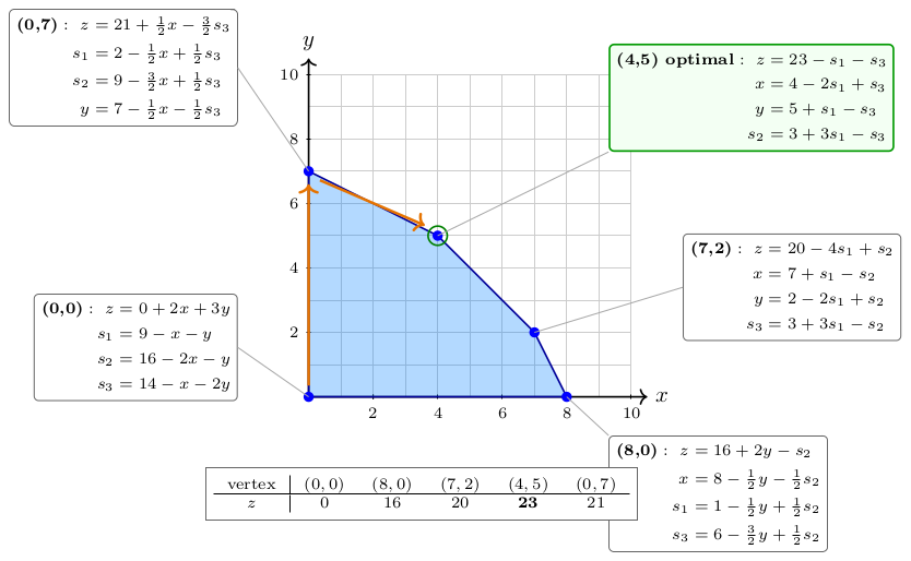
A useful way to internalize what just happened: every vertex of the feasible region has its own dictionary, the same linear program rewritten from that vertex’s point of view. Figure 7.4 shows all five dictionaries for our example. The simplex method simply walks from dictionary to dictionary along edges of the region, and the signs of the objective-row coefficients at each vertex tell it where to go next. At $(4, 5)$ both coefficients are negative, so the walk stops: no neighboring vertex is better.

Figure 7.4: The same linear program seen from every vertex: each basic feasible solution has its own dictionary, whose objective row reveals whether a better neighbor exists. The orange arrows trace the pivots taken in the text, $(0, 0) \to (0, 7) \to (4, 5)$ ; at $(4, 5)$ all objective coefficients are negative, certifying optimality.

7.4 The Simplex Algorithm!

Here we formally describe the simplex algorithm.

Algorithm: Simplex Method

Input. A linear program in standard form with a feasible starting basis (typically the slack variables).
Initialization. Write the system in dictionary form (basic variables on the left, nonbasic variables on the right) and substitute the basic variables into the objective function.

☞ Choose the entering variable Select a nonbasic variable with a positive coefficient in the objective row. (If no coefficient is positive, the current solution is already optimal.)

✏ Determine the leaving variable For each basic variable with a positive entering-variable coefficient, compute the ratio $\frac{current value of basic variable}{coefficient of entering variable}$ . The basic variable with the smallest ratio reaches zero first and leaves the basis.

❒ Pivot Rewrite the leaving variable’s equation so it is expressed in terms of the entering variable, then substitute this expression into all other equations and the objective function.

✔ Repeat until optimal Repeat the three steps above until every objective-row coefficient of a nonbasic variable is non-positive. The current basic solution is then optimal.

We dive a little deeper into what the ratio test is here:

The Ratio Test (Formal Definition)

The Ratio Test is used to determine which basic variable should leave the basis when a nonbasic variable enters. It ensures that we maintain feasibility by preventing any basic variables from becoming negative.

Given a pivot column corresponding to the entering variable (say, $x_{e}$ ), the Ratio Test is defined as follows:

Identify all constraints of the form:

s_{i} = b_{i} - a_{i, e} x_{e}

where $b_{i}$ is the right-hand side value, and $a_{i, e}$ is the coefficient of the entering variable in row $i$ .

Compute the ratio for all constraints where $a_{i, e} > 0$ :

$\frac{b_{i}}{a_{i, e}}$
The leaving variable corresponds to the row that gives the smallest positive ratio. This ensures that the increase in $x_{e}$ does not cause any basic variable to become negative.

Special Cases:

If all $a_{i, e} \leq 0$ , then the problem is unbounded, meaning the objective function can be increased indefinitely.
If multiple rows attain the same minimum ratio, a tie-breaking rule is needed (e.g., Bland’s Rule to avoid cycling).

The Ratio Test guarantees that we always select the proper constraint to maintain feasibility while pivoting towards an improved solution.

Learning Checkpoint 7.4.1

When applying the simplex method, why might choosing the wrong leaving variable during the ratio test lead you to an infeasible basic solution?

Hint: Think about what the ratio test is meant to guarantee for the nonnegativity of variables after the pivot.

We will see another example of this, and then modify it to handle LPs that don’t have a simple initial basic feasible solution.

7.4.1 Simplex Algorithm Execution

Here is the same computation from Section 7.3 again, this time in compact form, so you can see the whole run at a glance now that each step has a name. Each computation is colour-coded to match the algorithm card above: entering (green), ratio test / leaving (orange), pivot (blue), and optimal (purple).

Initial dictionary (basis ${s_{1}, s_{2}, s_{3}}$ ; nonbasic $x = y = 0$ ):

\begin{aligned} \max & z = 2 x + 3 y \\ s.t. & s_{1} = 9 - x - y \\ s_{2} = 16 - 2 x - y \\ s_{3} = 14 - x - 2 y \end{aligned}

Iteration 1.

☞ Entering. Both $x$ and $y$ have positive coefficients in $z = 2 x + 3 y$ . By steepest ascent we increase the one with the larger coefficient, $y$ (coefficient $3$ ), so $y$ enters.

✏ Ratio test. As $y$ increases (with $x = 0$ ), each basic variable stays nonnegative only up to its ratio:

$\begin{aligned} s_{1} = 9 - y & \geq 0 \Leftrightarrow y \leq 9 ∕ 1 = 9, \\ s_{2} = 16 - y & \geq 0 \Leftrightarrow y \leq 16 ∕ 1 = 16, \\ s_{3} = 14 - 2 y & \geq 0 \Leftrightarrow y \leq 14 ∕ 2 = 7 (smallest) . \end{aligned}$

The smallest ratio is $7$ , attained by $s_{3}$ , so $s_{3}$ leaves.

❒ Pivot. Solve the $s_{3}$ row for $y$ : $y = 7 - 0.5 x - 0.5 s_{3}$ . Substituting into the objective and the other rows gives

$\begin{aligned} \max & z = 21 + 0.5 x - 1.5 s_{3} \\ s.t. & s_{1} = 2 - 0.5 x + 0.5 s_{3} \\ s_{2} = 9 - 1.5 x + 0.5 s_{3} \\ y = 7 - 0.5 x - 0.5 s_{3} \end{aligned}$

Iteration 2.

☞ Entering. Only $x$ has a positive objective coefficient ( $0.5$ ), so $x$ enters.

✏ Ratio test. As $x$ increases (with $s_{3} = 0$ ):

$\begin{aligned} s_{1} = 2 - 0.5 x & \geq 0 \Leftrightarrow x \leq 2 ∕ 0.5 = 4 (smallest), \\ s_{2} = 9 - 1.5 x & \geq 0 \Leftrightarrow x \leq 9 ∕ 1.5 = 6, \\ y = 7 - 0.5 x & \geq 0 \Leftrightarrow x \leq 7 ∕ 0.5 = 14 . \end{aligned}$

The smallest ratio is $4$ , attained by $s_{1}$ , so $s_{1}$ leaves.

❒ Pivot. Solve the $s_{1}$ row for $x$ : $x = 4 - 2 s_{1} + s_{3}$ . Substituting gives

$\begin{aligned} \max & z = 23 - s_{1} - s_{3} \\ s.t. & x = 4 - 2 s_{1} + s_{3} \\ s_{2} = 3 + 3 s_{1} - s_{3} \\ y = 5 + s_{1} - s_{3} \end{aligned}$

✔ Optimal. Every nonbasic objective coefficient is $\leq 0$ , so no further improvement is possible: $x = 4, y = 5, z = 23$ .

In the example worked out in the prior section, we used the steepest ascent pivot rule, which means that we always used the variable in the objective with the largest positive coefficient to enter the basis. However, we could make other choices instead. The choice of how to pivot is left a little ambiguous in the simplex method and many different pivot rules have been proposed. See Exercise 7.25 to see how the simplex method plays out when pivoting in a different direction first.

In fact, in the figure below, we show the simplex dictionary at every single vertex. You can see that from any vertex, you can pivot along an edge of the feasible region to another vertex.

Figure 7.5: The feasible region with the basis and objective value at every vertex; the simplex path leads to...

Remark. Reduced Costsdef:reduced-cost The coefficients of the nonbasic variables in the objective row are their reduced costs:

Reduced cost of s_{1} = - 1, Reduced cost of s_{3} = - 1 .

\begin{aligned} \max & z = 23 - s_{1} - s_{3} \\ s.t. & x = 4 - 2 s_{1} + s_{3}, \\ y = 5 + s_{1} - s_{3}, \\ s_{2} = 3 + 3 s_{1} - s_{3}, \\ x, y, s_{1}, s_{2}, s_{3} \geq 0 . \end{aligned}

These values indicate how much the objective $z$ would change per unit increase in the corresponding variable, assuming all others are held fixed and feasibility is maintained.
Because this is a maximization problem, a negative reduced cost implies that increasing the variable would decrease the objective.

Optimality Condition: A basic feasible solution is optimal if and only if all reduced costs of nonbasic variables satisfy:

(for maximization): reduced cost \leq 0 .

In this dictionary:

Reduced costs of s_{1}, s_{3} < 0 \Rightarrow no nonbasic variable can enter to improve z .

Therefore, the current solution is optimal.

Definition 7.14: Reduced Costs in an Arbitrary Dictionary

Let a linear program in standard form be given by

\max c^{⊤} x s.t. A x = b, x \geq 0,

and let $B \subseteq {1, \dots, n}$ be a basis of linearly independent columns of $A$ . The corresponding dictionary expresses the basic and objective variables in terms of the nonbasic variables $N = {1, \dots, n} ∖ B$ :

\begin{aligned} z & = z_{0} + \sum_{j \in N} {\bar{c}}_{j} x_{j} \\ x_{i} & = {\bar{b}}_{i} + \sum_{j \in N} ā_{i j} x_{j} for i \in B \end{aligned}

Here:

$x_{i}$ are the basic variables,
$x_{j}$ for $j \in N$ are the nonbasic variables,
$z_{0}$ is the current value of the objective,
${\bar{c}}_{j}$ is the reduced cost of variable $x_{j}$ , and
${\bar{b}}_{i}$ is the value of basic variable $x_{i}$ when $x_{j} = 0$ for all $j \in N$ .

7.5 No Feasible Initial Basis and the Big-M Method

Try it out visually!

Two-Phase Simplex: watch artificial variables enter, Phase 1 drive them out, and the handoff to Phase 2.

Learning Outcomes

Address case where initial basis is infeasible
Modify the simplex algorithm using the Big-M method to find a feasible starting basis
- Introduce artificial variables to rows that violate initial feasibility
- Add large penalty (Big-M) to the objective on these artificial variables
- Run Simplex and pivot until can remove artificial variables
- Drop the auxiliary variables and proceed with the simplex algorithm

Every worked example so far started from the origin $x = y = 0$ , where the slack variables handed us an obvious basic feasible solution. That convenience disappears the moment the problem has a “ $\geq$ ” constraint: at the origin the corresponding slack is negative, so the natural starting dictionary is infeasible and there is no basis from which to launch the simplex method. This section shows how to manufacture a feasible starting basis with an artificial variable penalized by a large constant $M$ (the Big-M method), and how the same device reveals when a problem has no feasible solution at all.

Consider

\begin{aligned} \max & 2 x + 3 y \\ s.t. & 2 x + y \geq 5, \\ 2 x + y \leq 16, \\ x + 2 y \leq 14, \\ x, y \geq 0 . \end{aligned}

The first constraint points the wrong way for an easy start, so the origin is infeasible and we cannot simply read off a starting basis.

Geometrically, the origin lies outside the feasible region, so it cannot serve as a starting vertex:

Figure 7.6: Feasible region after adding the constraint 2x+y>=5: the pink triangle near the origin becomes infeasible.

Step 1 — Put every constraint in “ $\leq$ ” form. Multiplying the $\geq$ constraint by $- 1$ turns it into a $\leq$ constraint:

$\begin{aligned} \max & 2 x + 3 y \\ s.t. & - 2 x - y \leq - 5, \\ 2 x + y \leq 16, \\ x + 2 y \leq 14, \\ x, y \geq 0 . \end{aligned}$

Step 2 — Form the slack dictionary and spot the infeasibility. Introducing slack variables gives

$\begin{aligned} \max & 2 x + 3 y \\ s.t. & s_{1} = - 5 + 2 x + y, \\ s_{2} = 16 - 2 x - y, \\ s_{3} = 14 - x - 2 y, \\ x, y, s_{1}, s_{2}, s_{3} \geq 0 . \end{aligned}$

At $x = y = 0$ this gives $s_{1} = - 5 < 0$ , so the dictionary is infeasible and the usual simplex start is unavailable.

Step 3 — Introduce an artificial variable. Add a nonnegative artificial variable $a_{1}$ to the offending equation and penalize it heavily in the objective (here $M = 1000$ ), so the simplex method is driven to push it back to zero:

$\begin{aligned} \max & 2 x + 3 y - 1000 a_{1} \\ s.t. & s_{1} = - 5 + 2 x + y + a_{1}, \\ s_{2} = 16 - 2 x - y, \\ s_{3} = 14 - x - 2 y, \\ x, y, s_{1}, s_{2}, s_{3}, a_{1} \geq 0 . \end{aligned}$

Step 4 — Pivot to a feasible basis. Swapping $a_{1}$ into the basis in place of $s_{1}$ makes every right-hand side nonnegative at $x = y = 0$ , giving a genuine starting point:

$\begin{aligned} \max & - 5000 + 2002 x + 1003 y - 1000 s_{1} \\ s.t. & a_{1} = 5 - 2 x - y + s_{1}, \\ s_{2} = 16 - 2 x - y, \\ s_{3} = 14 - x - 2 y, \\ x, y, s_{1}, s_{2}, s_{3}, a_{1} \geq 0 . \end{aligned}$

With a feasible basis in hand, we run the simplex method as usual. Letting $x$ enter drives the artificial variable back out of the basis:

\begin{aligned} \max & 5 + 2 y + s_{1} - 1001 a_{1} \\ s.t. & x = 2.50 - 0.50 y + 0.50 s_{1} - 0.50 a_{1}, \\ s_{2} = 11 - s_{1} + a_{1}, \\ s_{3} = 11.50 - 1.50 y - 0.50 s_{1} + 0.50 a_{1}, \\ x, y, s_{1}, s_{2}, s_{3}, a_{1} \geq 0 . \end{aligned}

The structure of this feasible dictionary is worth pausing on.

Remark. Artificial Variable Can Be Removed: Feasible Start for Phase II This is the second artificial dictionary from Phase I of the two-phase simplex method. Our goal was to eliminate the artificial variable $a_{1}$ while finding a feasible solution to the original problem.

Consider this dictionary:

The artificial variable $a_{1}$ appears in the system, but it is not basic.
Because $a_{1}$ is a nonbasic variable and its value is currently zero, it can be removed from the dictionary without violating feasibility.
All basic variables ( $x, s_{2}, s_{3}$ ) have nonnegative values when $a_{1} = 0$ , and all coefficients of $a_{1}$ can simply be deleted.

Conclusion: We now have a basic feasible solution to the original problem (with no artificial variables present), so we can begin Phase II of the simplex method using this dictionary as the starting point.

\begin{aligned} \max & 5 + 2 y + s_{1} - 1001 a_{1} \\ s.t. & x = 2.50 - 0.50 y + 0.50 s_{1} - 0.50 a_{1}, \\ s_{2} = 11 - s_{1} + a_{1}, \\ s_{3} = 11.50 - 1.50 y - 0.50 s_{1} + 0.50 a_{1}, \\ x, y, s_{1}, s_{2}, s_{3}, a_{1} \geq 0 . \end{aligned}

Learning Checkpoint 7.5.1

Why can the artificial variable be removed from this system?

Now $a_{1}$ is nonbasic, so the basis is feasible for the original problem. We may discard the artificial variable and continue from the feasible dictionary

\begin{aligned} \max & 5 + 2 y + s_{1} \\ s.t. & x = 2.50 - 0.50 y + 0.50 s_{1}, \\ s_{2} = 11 - s_{1}, \\ s_{3} = 11.50 - 1.50 y - 0.50 s_{1}, \\ x, y, s_{1}, s_{2}, s_{3} \geq 0 . \end{aligned}

7.5.1 Big-M Method Algorithm

Algorithm: Big-M Method

Input. A linear program in standard form (maximize), possibly with an infeasible initial basic solution.

☞ Add artificial variables For each constraint with a negative right-hand side, multiply the constraint by $- 1$ so the RHS becomes positive. For each constraint without an obvious feasible basic variable, add an artificial variable $a_{i} \geq 0$ .

✏ Penalize the artificials Add a penalty term $- M a_{i}$ (with $M$ a very large constant) for each artificial variable to the objective. Form the initial dictionary (including slack/surplus and artificial variables) using this modified objective, with the artificials in the starting basis.

❒ Drive the artificials out While an artificial variable is in the basis (or the basic solution is infeasible), perform a simplex pivot, using the modified objective, that moves at least one artificial variable out of the basis.

☞ Restore and continue Once all artificial variables are zero, remove their columns and continue the standard simplex iterations using the original objective function.

✔ Output The optimal solution to the original problem, or a declaration of infeasibility if any artificial variable remains positive.

7.5.2 Detecting Infeasibility via the Big-M Method

Consider the linear program

\begin{aligned} \max & 2 x + 3 y \\ s.t. & 2 x + y \geq 22, 2 x + y \leq 16, x + 2 y \leq 14, x, y \geq 0 . \end{aligned}

The first two constraints demand that $2 x + y$ be simultaneously at least $22$ and at most $16$ , so we should expect trouble. Rewriting the $\geq$ constraint as $- 2 x - y \leq - 22$ and adding a slack gives $s_{1} = - 22 + 2 x + y$ , which is negative at the origin. Exactly as before, we add an artificial variable $a_{1}$ (penalty $M = 1000$ ) and pivot it into the basis to obtain a feasible starting dictionary:

$\begin{aligned} \max & - 22000 + 2002 x + 1003 y - 1000 s_{1} \\ s.t. & a_{1} = 22 - 2 x - y + s_{1}, \\ s_{2} = 16 - 2 x - y, \\ s_{3} = 14 - x - 2 y . \end{aligned}$

Pivot: $x$ enters, $s_{2}$ leaves.

$\begin{aligned} \max & - 5984 + 2 y - 1000 s_{1} - 1001 s_{2} \\ s.t. & a_{1} = 6 + s_{1} + s_{2}, \\ x = 8 - 0.50 y - 0.50 s_{2}, \\ s_{3} = 6 - 1.50 y + 0.50 s_{2} . \end{aligned}$

Pivot: $y$ enters, $s_{3}$ leaves.

$\begin{aligned} \max & - 5976 - 1000 s_{1} - 1000.33 s_{2} - 1.33 s_{3} \\ s.t. & a_{1} = 6 + s_{1} + s_{2}, \\ x = 6 - 0.67 s_{2} + 0.33 s_{3}, \\ y = 4 + 0.33 s_{2} - 0.67 s_{3} . \end{aligned}$

Every objective-row coefficient is now nonpositive, so this dictionary is optimal for the penalized (Big-M) problem, yet the artificial variable is still basic.

Interpreting the Final Dictionary

In the final dictionary, the artificial variable $a_{1}$ appears in the equation

a_{1} = 6 + s_{1} + s_{2} .

When the nonbasic variables $s_{1}$ and $s_{2}$ are set to zero (which is typical in a basic solution), we find

a_{1} = 6 .

Because $a_{1} > 0$ in the optimal dictionary, this indicates that the original linear program has no feasible solution. The presence of a positive artificial variable in the final optimal dictionary is the standard signal in the Big-M method that the original problem is infeasible.

In summary, the contradictory constraints (requiring $2 x + y$ to be both at least 22 and at most 16) force the artificial variable $a_{1}$ to remain positive. Thus, the Big-M method confirms that the problem is infeasible.

Remark. Final Artificial Dictionary Indicates Infeasibility This is the final dictionary at the end of Phase I of the two-phase simplex method, where the goal was to eliminate the artificial variable $a_{1}$ and reach a feasible solution to the original problem.

To interpret this:

The artificial variable $a_{1}$ is still in the basis.
Its value is expressed as $a_{1} = 6 + s_{1} + s_{2}$ , and since all variables on the right-hand side are constrained to be nonnegative, we have $a_{1} \geq 6$ .
Therefore, we cannot make $a_{1} = 0$ , which is required to reach feasibility in Phase I.

Thus, there is no feasible solution to the original problem.
Conclusion: The original linear program is infeasible.

\begin{aligned} \max & - 5976 - 1000 s_{1} - 1000.33 s_{2} - 1.33 s_{3} \\ s.t. & a_{1} = 6 + s_{1} + s_{2}, \\ x = 6 - 0.67 s_{2} + 0.33 s_{3}, \\ y = 4 + 0.33 s_{2} - 0.67 s_{3}, \\ x, y, s_{1}, s_{2}, s_{3}, a_{1} \geq 0 . \end{aligned}

Theorem 7.15: Infeasibility Detection via the Big-M Method

Consider the linear programming problem

\begin{aligned} \max & c^{⊤} x \\ s.t. & A x \leq b, \\ x \geq 0 . \end{aligned}

After converting inequalities to equalities by introducing slack, surplus, and, if needed, artificial variables, the system takes the form

A x - I_{a} a = b, x, a \geq 0,

where $I_{a}$ is a submatrix of the identity matrix, with each column corresponding to an artificial variable introduced to enforce equality in a constraint that initially lacked a basic variable with a nonnegative right-hand side. The Big-M formulation is then given by

\max c^{⊤} x - M \sum_{i \in I} a_{i} .

If, in any optimal solution of the Big-M problem, there exists an artificial variable $a_{i} > 0$ for some $i \in I$ , then the original linear programming problem is infeasible.

Proof. Assume that an optimal solution $(x^{*}, a^{*})$ of the Big-M problem satisfies $a_{i}^{*} > 0$ for some $i \in I$ .

Suppose, for contradiction, that the original linear programming problem is feasible. Then there exists some $x^{'} \geq 0$ such that $A x^{'} \leq b$ . In the reformulation process, if a constraint lacked a basic variable with a nonnegative right-hand side, an artificial variable $a_{i}$ was introduced, rewriting the constraint as

(original constraint) - a_{i} = b_{i} .

For any feasible $x^{'}$ of the original problem, we can set $a^{'} = 0$ for all artificial variables, and the equality constraints will still be satisfied.

Thus, the solution $(x^{'}, 0)$ is feasible for the Big-M formulation, and its objective value is exactly $c^{⊤} x^{'}$ . On the other hand, the optimal solution $(x^{*}, a^{*})$ yields an objective value of

c^{⊤} x^{*} - M \sum_{i \in I} a_{i}^{*} .

Since $M$ is chosen to be a very large positive constant, any positive contribution from $\sum_{i \in I} a_{i}^{*}$ imposes a severe penalty. Consequently, the objective value of $(x^{'}, 0)$ would be strictly greater than that of $(x^{*}, a^{*})$ provided that $M$ is sufficiently large.

This contradiction implies that no feasible solution $(x^{'}, 0)$ exists for the original problem. In other words, the assumption that the original problem is feasible is false.

Hence, if in the optimal solution of the Big-M problem any artificial variable remains positive, the original linear programming problem must be infeasible. □

7.5.3 A second example: two artificial variables

When several constraints point the “wrong” way, we simply add one artificial variable per offending constraint. Consider

\begin{aligned} \max & 3 x + y \\ s.t. & 2 x + y \geq 5, 2 x + y \leq 16, x + 2 y \geq 3, x, y \geq 0 . \end{aligned}

Two constraints are of “ $\geq$ ” type, so the origin violates both. Flipping them to $- 2 x - y \leq - 5$ and $- x - 2 y \leq - 3$ and adding slacks gives $s_{1} = - 5 + 2 x + y$ and $s_{3} = - 3 + x + 2 y$ , both negative at the origin. We introduce two artificial variables $a_{1}, a_{3}$ (each penalized by $M = 1000$ ) and pivot them into the basis, producing a feasible starting dictionary whose objective row carries the Big-M penalty:

$\begin{aligned} \max & - 8000 + 3003 x + 3001 y - 1000 s_{1} - 1000 s_{3} \\ s.t. & a_{1} = 5 - 2 x - y + s_{1}, \\ s_{2} = 16 - 2 x - y, \\ a_{3} = 3 - x - 2 y + s_{3} . \end{aligned}$

The large penalties make $x$ and $y$ attractive to increase, and successive pivots drive both artificial variables out of the basis. Once $a_{1} = a_{3} = 0$ the basis is feasible for the original problem; we drop the artificials and continue on the true objective $3 x + y$ until every reduced cost is nonpositive:

$\begin{aligned} \max & 24 - 0.5 y - 1.5 s_{2} \\ s.t. & x = 8 - 0.5 y - 0.5 s_{2}, \\ s_{1} = 11 - s_{2}, \\ s_{3} = 5 + 1.5 y - 0.5 s_{2} . \end{aligned}$

Reading the optimal dictionary gives $x = 8$ , $y = 0$ , and $z = 3 x + y = 24$ , with the first and third constraints slack ( $s_{1} = 11$ , $s_{3} = 5$ ) and the second constraint tight ( $s_{2} = 0$ ).

7.6 Degeneracy, Cycling, and Bland’s Rule

Definition 7.16: Degeneracy

A basic feasible solution (BFS) in the Simplex Method is said to be degenerate if one or more of its basic variables take a value of zero. Mathematically, a BFS corresponding to a basis $B$ is degenerate if there exists at least one basic variable $x_{B}$ such that $x_{B} = 0$ .

Remark. Degenerate Dictionary The dictionary below represents a feasible solution, but one of the basic variables is equal to zero. This situation is called degeneracy.

What is degeneracy? A dictionary is called degenerate if any basic variable is equal to zero. This is important because:

It can cause the simplex method to perform a pivot without changing the objective value.
It can potentially lead to cycling, revisiting the same basic solution more than once.

In this dictionary:

The basic variables are $x_{3}, x_{4}, x_{5}, x_{6}$ .

When we set the nonbasic variables $x_{1} = 0$ , $x_{2} = 0$ , we find:

x_{3} = 4, x_{4} = 2, x_{5} = 3, x_{6} = 0, z = 0 .

Since $x_{6} = 0$ and it is in the basis, this is a degenerate basic feasible solution.

\begin{aligned} \max & z = 0 + x_{1} + 2 x_{2} \\ s.t. & x_{3} = 4 - x_{2}, \\ x_{4} = 2 - x_{1} + x_{2}, \\ x_{5} = 3 - x_{1}, \\ x_{6} = 0 + 2 x_{1} - x_{2}, \\ x_{1}, x_{2}, x_{3}, x_{4}, x_{5}, x_{6} \geq 0 . \end{aligned}

In this case, the basic feasible solution is (basic variables) $(x_{3}, x_{4}, x_{5}, x_{6}) = (4, 2, 3, 0)$ and (non-basic variables) $(x_{1}, x_{2}) = (0, 0)$ .

7.6.1 Degeneracy and Unchanged BFS after Pivoting

Degeneracy can lead to cases where pivoting in the Simplex Method does not change the basic feasible solution. When a pivot is performed, the entering variable is increased until one of the current basic variables reaches zero, at which point that variable leaves the basis. However, if multiple constraints yield the same minimum ratio in the ratio test, then a tie-breaking rule must be applied. If the variable that leaves the basis was already zero, the BFS remains unchanged.

Notice in the prior example, we can try to let $x_{2}$ enter the basis. What happens? By the ratio test, we see that $x_{6}$ leaves the basis. This results in the following new dictionary:

Remark. Degenerate Pivot: No Change in BFS After pivoting $x_{2}$ into the basis and $x_{6}$ out, we arrive at the dictionary below.

Here is what happened:

Before the pivot, the basic variables were $x_{3}, x_{4}, x_{5}, x_{6}$ , and the nonbasic variables were $x_{1} = 0, x_{2} = 0$ .
After the pivot, $x_{2}$ enters and $x_{6}$ leaves. The new basic variables are $x_{3}, x_{4}, x_{5}, x_{2}$ .

However, when we plug in the nonbasic values $x_{1} = 0, x_{6} = 0$ , we get:

x_{3} = 4, x_{4} = 2, x_{5} = 3, x_{2} = 0, z = 0 .

This is identical to the previous basic feasible solution.

Conclusion: This is a case of a degenerate pivot: we performed a pivot step, but the resulting basic feasible solution did not change. The simplex algorithm moved to a new dictionary (i.e., a new basis), but the point in solution space stayed the same.

\begin{aligned} \max & z = 0 + 5 x_{1} - 2 x_{6} \\ s.t. & x_{3} = 4 - 2 x_{1} + x_{6}, \\ x_{4} = 2 + x_{1} - x_{6}, \\ x_{5} = 3 - x_{1}, \\ x_{2} = 0 + 2 x_{1} - x_{6}, \\ x_{1}, x_{2}, x_{3}, x_{4}, x_{5}, x_{6} \geq 0 . \end{aligned}

But! The basic feasible solution is the same!!!

Fortunately, the next pivot leads to a new solution.

However, this phenomenon can cause the algorithm to visit the same BFS multiple times, potentially leading to cycling.

See https://gilp.henryrobbins.com/en/latest/examples/3d/SQUARE_PYRAMID_3D_LP.html for a highly degenerate case where the first two pivots do not change the solution.

7.7 Cycling in the Simplex Method

In the Simplex Method, a pivot operation normally improves the objective function by moving from one basic feasible solution (BFS) to another. However, in rare cases, the method can revisit the same BFS multiple times without progress. This phenomenon is called cycling.

Cycling occurs due to:

Degeneracy: when one or more basic variables are zero.
Unlucky pivot rules: which cause the algorithm to rotate through different bases that correspond to the same BFS.

The following example demonstrates cycling. The entering variable is chosen by the largest-coefficient rule, and ties in the minimum ratio test are broken naively, by taking the tied row whose basic variable is listed first. This combination cycles on the example below. Anti-cycling pivot rules, such as the lexicographic rule or Bland’s rule (described later in this section), prevent this behavior.

7.7.1 Cycling in the Simplex Method

Cycling occurs when the Simplex Method revisits the same set of basic variables repeatedly without making progress in improving the objective function. This happens when degeneracy is present and the choice of entering and leaving variables results in looping between a set of degenerate BFSs.

The following example demonstrates cycling in the Simplex Method. It is a rescaled version of the classic cycling example constructed by E. M. L. Beale (1955), the first published instance of an LP on which the simplex method cycles; only the units of two variables have been changed, which preserves the cycle.

Initial Dictionary

\begin{aligned} \max & z = 0 + 0.75 x_{1} - 20 x_{2} + 0.50 x_{3} - 6 x_{4} \\ s.t. & s_{1} = 0 - 0.25 x_{1} + 8 x_{2} + x_{3} - 9 x_{4}, \\ s_{2} = 0 - 0.50 x_{1} + 12 x_{2} + 0.50 x_{3} - 3 x_{4}, \\ s_{3} = 1 - x_{3}, \\ x_{1}, x_{2}, x_{3}, x_{4}, s_{1}, s_{2}, s_{3} \geq 0 . \end{aligned}

Pivot: $x_{1}$ enters, $s_{1}$ leaves.

\begin{aligned} \max & z = 0 + 4 x_{2} + 3.50 x_{3} - 33 x_{4} - 3 s_{1} \\ s.t. & x_{1} = 0 + 32 x_{2} + 4 x_{3} - 36 x_{4} - 4 s_{1}, \\ s_{2} = 0 - 4 x_{2} - 1.50 x_{3} + 15 x_{4} + 2 s_{1}, \\ s_{3} = 1 - x_{3}, \\ x_{1}, x_{2}, x_{3}, x_{4}, s_{1}, s_{2}, s_{3} \geq 0 . \end{aligned}

Pivot: $x_{2}$ enters, $s_{2}$ leaves.

\begin{aligned} \max & z = 0 + 2 x_{3} - 18 x_{4} - s_{1} - s_{2} \\ s.t. & x_{1} = 0 - 8 x_{3} + 84 x_{4} + 12 s_{1} - 8 s_{2}, \\ x_{2} = 0 - 0.38 x_{3} + 3.75 x_{4} + 0.50 s_{1} - 0.25 s_{2}, \\ s_{3} = 1 - x_{3}, \\ x_{1}, x_{2}, x_{3}, x_{4}, s_{1}, s_{2}, s_{3} \geq 0 . \end{aligned}

Pivot: $x_{3}$ enters, $x_{1}$ leaves.

\begin{aligned} \max & z = 0 - 0.25 x_{1} + 3 x_{4} + 2 s_{1} - 3 s_{2} \\ s.t. & x_{3} = 0 - 0.12 x_{1} + 10.50 x_{4} + 1.50 s_{1} - s_{2}, \\ x_{2} = 0 + 0.05 x_{1} - 0.19 x_{4} - 0.06 s_{1} + 0.12 s_{2}, \\ s_{3} = 1 + 0.12 x_{1} - 10.50 x_{4} - 1.50 s_{1} + s_{2}, \\ x_{1}, x_{2}, x_{3}, x_{4}, s_{1}, s_{2}, s_{3} \geq 0 . \end{aligned}

Pivot: $x_{4}$ enters, $x_{2}$ leaves.

\begin{aligned} \max & z = + 0.50 x_{1} - 16 x_{2} + s_{1} - s_{2} \\ s.t. & x_{3} = 0 + 2.50 x_{1} - 56 x_{2} - 2 s_{1} + 6 s_{2}, \\ x_{4} = 0 + 0.25 x_{1} - 5.33 x_{2} - 0.33 s_{1} + 0.67 s_{2}, \\ s_{3} = 1 - 2.50 x_{1} + 56 x_{2} + 2 s_{1} - 6 s_{2}, \\ x_{1}, x_{2}, x_{3}, x_{4}, s_{1}, s_{2}, s_{3} \geq 0 . \end{aligned}

Pivot: $s_{1}$ enters, $s_{3}$ leaves.

\begin{aligned} \max & z = + 1.75 x_{1} - 44 x_{2} - 0.50 x_{3} + 2 s_{2} \\ s.t. & s_{1} = 0 + 1.25 x_{1} - 28 x_{2} - 0.50 x_{3} + 3 s_{2}, \\ x_{4} = 0 - 0.17 x_{1} + 4 x_{2} + 0.17 x_{3} - 0.33 s_{2}, \\ s_{3} = 1 - x_{3}, \\ x_{1}, x_{2}, x_{3}, x_{4}, s_{1}, s_{2}, s_{3} \geq 0 . \end{aligned}

Pivot: $s_{2}$ enters, $x_{4}$ leaves.

\begin{aligned} \max & z = + 0.75 x_{1} - 20 x_{2} + 0.50 x_{3} - 6 x_{4} \\ s.t. & s_{1} = 0 - 0.25 x_{1} + 8 x_{2} + x_{3} - 9 x_{4}, \\ s_{2} = 0 - 0.50 x_{1} + 12 x_{2} + 0.50 x_{3} - 3 x_{4}, \\ s_{3} = 1 - x_{3}, \\ x_{1}, x_{2}, x_{3}, x_{4}, s_{1}, s_{2}, s_{3} \geq 0 . \end{aligned}

This last dictionary is identical to the initial one: after six pivots the method has returned to its starting basis with the objective still at $z = 0$ . The simplex method is cycling, and without an anti-cycling safeguard it will loop forever.

7.7.2 Bland’s Rule

Bland’s Rule is a tie-breaking strategy used to prevent cycling in the Simplex Method. The rule ensures that:

1.: The variable with the smallest index enters the basis when multiple choices exist.
2.: The variable with the smallest index leaves the basis when multiple choices exist.

By enforcing this lexicographic ordering, the method guarantees progress and prevents the algorithm from revisiting the same basis indefinitely.

Theorem 7.17: Bland’s Rule Prevents Cycling

If Bland’s Rule is used to select the entering and leaving variables in the Simplex Method, then the algorithm will terminate in a finite number of steps, either by reaching an optimal solution or by detecting an unbounded problem.

Proof sketch. Suppose, for contradiction, that the method cycles: a sequence of degenerate pivots returns to a basis visited before. During a cycle the basic feasible solution and the objective value never change, and some set of variables enters and leaves the basis over and over. Consider the largest-indexed variable $x_{t}$ that takes part in the cycle. Comparing the dictionary at a step where $x_{t}$ enters with the dictionary at a step where $x_{t}$ leaves, a sign analysis of the two objective rows shows that at one of these steps some variable with index smaller than $t$ was also eligible, so Bland’s rule could not have selected $x_{t}$ there, a contradiction. Hence no basis repeats; since there are finitely many bases, the algorithm terminates. The full argument is standard and can be found, for example, in Chvátal’s Linear Programming. □

From the example above, following the same sequence, we arrive at this dictionary.

\begin{aligned} \max & z = + 0.50 x_{1} - 16 x_{2} + s_{1} - s_{2} \\ s.t. & x_{3} = 0 + 2.50 x_{1} - 56 x_{2} - 2 s_{1} + 6 s_{2}, \\ x_{4} = 0 + 0.25 x_{1} - 5.33 x_{2} - 0.33 s_{1} + 0.67 s_{2}, \\ s_{3} = 1 - 2.50 x_{1} + 56 x_{2} + 2 s_{1} - 6 s_{2}, \\ x_{1}, x_{2}, x_{3}, x_{4}, s_{1}, s_{2}, s_{3} \geq 0 . \end{aligned}

Pivot: $x_{1}$ enters, $s_{3}$ leaves. Bland’s rule: choose the lowest-index eligible entering and leaving variables

\begin{aligned} \max & z = 0.20 - 4.80 x_{2} + 1.40 s_{1} - 2.20 s_{2} - 0.20 s_{3} \\ s.t. & x_{3} = 1 - s_{3}, \\ x_{4} = 0.10 + 0.27 x_{2} - 0.13 s_{1} + 0.07 s_{2} - 0.10 s_{3}, \\ x_{1} = 0.40 + 22.40 x_{2} + 0.80 s_{1} - 2.40 s_{2} - 0.40 s_{3}, \\ x_{1}, x_{2}, x_{3}, x_{4}, s_{1}, s_{2}, s_{3} \geq 0 . \end{aligned}

Bland’s rule breaks the tie differently from before: the method moves to a genuinely new basis and the objective strictly increases to $z = 0.20$ . The cycle is broken, and the simplex method now makes progress toward optimality.

7.8 Simplex and Unbounded LPs

Example 7.18: Unbounded Linear Program

Consider the linear program:

\begin{aligned} maximize & x_{1} \\ s.t. & x_{1} - x_{2} \leq 1 \\ 2 x_{1} - x_{2} \leq 3 \\ x_{1}, x_{2} \geq 0 \end{aligned}

Figure 7.7: Desmos plot of the feasible region defined by x1-x2<=1, 2x1-x2<=3, x1,x2>=0: an unbounded region...

We convert the inequalities into equalities using slack variables $s_{1}$ and $s_{2}$ :

\begin{aligned} s_{1} & = 1 - x_{1} + x_{2} \\ s_{2} & = 3 - 2 x_{1} + x_{2} \\ x_{1}, x_{2}, s_{1}, s_{2} & \geq 0 \end{aligned}

Initial dictionary.

\begin{aligned} \max & z = x_{1} \\ s.t. & s_{1} = 1 - x_{1} + x_{2}, \\ s_{2} = 3 - 2 x_{1} + x_{2} . \end{aligned}

Pivot: $x_{1}$ enters, $s_{1}$ leaves. ratio test: $1 ∕ 1 < 3 ∕ 2$ , so $s_{1}$ leaves

\begin{aligned} \max & z = 1 + x_{2} - s_{1} \\ s.t. & x_{1} = 1 + x_{2} - s_{1}, \\ s_{2} = 1 - x_{2} + 2 s_{1} . \end{aligned}

Pivot: $x_{2}$ enters, $s_{2}$ leaves. only $s_{2}$ limits $x_{2}$

\begin{aligned} \max & z = 2 + s_{1} - s_{2} \\ s.t. & x_{1} = 2 + s_{1} - s_{2}, \\ x_{2} = 1 + 2 s_{1} - s_{2} . \end{aligned}

Now $s_{1}$ is eligible to enter (its objective coefficient $+ 1$ is positive), but its column is entirely nonnegative: in $x_{1} = 2 + s_{1} - s_{2}$ and $x_{2} = 1 + 2 s_{1} - s_{2}$ the coefficients of $s_{1}$ are $+ 1$ and $+ 2$ . Increasing $s_{1}$ raises both basic variables and never drives one to zero, so the ratio test finds no limiting row. The objective $z = 2 + s_{1}$ grows without bound, and the linear program is unbounded.

Conclusion: This linear program is unbounded. Once $s_{1}$ enters the basis, there is no constraint limiting how large it can grow while maintaining feasibility. Therefore, the objective function can increase without bound.

Pioneer Spotlight: George Dantzig

George Dantzig, known for spearheading linear programming with the simplex algorithm, was born in Portland, Oregon on November 8, 1914.¹ George received his Bachelor of Arts in Mathematics and Physics from the University of Maryland, College Park. After marrying his wife, Anne Shmuner, he completed his Master of Arts in Mathematics at the University of Michigan in 1938. Before graduating with his Master’s degree, he began working at the United States Bureau of Labor Statistics as a junior statistician. George took interest in statistics through the work of Jerzy Neyman, which led him to earn a Ph.D. in Statistics with Neyman’s guidance from the University of California, Berkeley in 1946. Before his dissertation, he began working with the Army Air Force Combat Analysis Branch of Statistical Control at the Pentagon, then transferred to the Department of the Air Force as a mathematical advisor. After his work at the Pentagon, he became a professor in operations research at the University of California, Berkeley, and Stanford. He went on to receive the National Medal of Science in 1975. He was also a member of the National Academy of Engineering, the National Academy of Sciences, and the American Association of Arts and Sciences.²

While in school at the University of California, Berkeley, George became widely known for solving two of the “unsolved” statistics problems, which he mistakenly thought were homework. In 1947, Dantzig proposed the simplex algorithm, which started the field of linear programming.³ Geometrically, the simplex method consists of traveling along the edges of a polyhedron from vertex to vertex. The feasible region of a linear program is always convex, and if the program has an optimal solution and its feasible region has a vertex, then some optimal solution occurs at a vertex. The linear program should be in the following standard form:

\max c^{⊤} x subject to A x = b, x \geq 0 .

The corresponding vertices of the feasible region are the basic feasible solutions. If a system is nondegenerate, the process of simplex pivoting can occur, where the previous solution is used to pivot towards a better feasible basis.

After Dantzig’s development of the simplex algorithm, he presented a talk geared toward the application of his linear programming model in the digital world, including games and computers. His algorithm was implemented in the animal feed industry and computing machines for the Air Force. It was also used to solve Stigler’s “diet problem,” a simple question with modern technology, but a long computation process in 1947. Dantzig’s procedure has been utilized in countless industries, such as communications, railroads, petroleum, airlines, and the economy. His utilization of linear algebra theory and the creation of pivoting will continue to be used when solving complex linear problems.

Dantzig also studied network flow problems, which led to the duality theorem in the 1950s. The dual theorem utilizes the costs as integers to create a pair that highlights integer basic solutions, which was used in the application of the “fleet assignment model.” With a great understanding of real-world problems, Dantzig developed the recourse stochastic program, which accounted for uncertain constraints and utilized statistical tests to determine the likelihood of an optimal solution. Dantzig was responsible for the solution to countless military problems through his development of linear programming in the late-1940s.

This spotlight was contributed by Irma Adams

7.9 Exercises

Warm-ups

Exercise 7.19: Standard form and the first dictionary

$⋆$ Consider the linear program

\begin{aligned} \max & 4 x + 5 y \\ s.t. & x + 2 y \leq 12, \\ 3 x + 2 y \leq 24, \\ x, y \geq 0 . \end{aligned}

1.: Convert the program to standard form by introducing slack variables $s_{1}, s_{2}$ .
2.

[§7.3, Initial Dictionary; §7.1]

Exercise 7.20: Convert to Standard Form

$⋆$ Convert the following linear program to standard form:

\begin{aligned} \max & 3 x_{1} - 5 x_{2} \\ s.t. & 2 x_{1} + x_{2} \leq 6, \\ - x_{1} + 3 x_{2} \geq 2, \\ x_{1}, x_{2} \geq 0 . \end{aligned}

[§7.1, Example: Complete Conversion to Standard Form]

Exercise 7.21: Convert to Standard Form

$⋆$ Convert the following linear program to standard form:

\begin{aligned} \min & - x_{1} + 2 x_{2} + x_{3} \\ s.t. & x_{1} - x_{2} + 2 x_{3} = 4, \\ - 2 x_{1} + x_{2} \leq 1, \\ x_{3} is unrestricted, x_{1}, x_{2} \geq 0 . \end{aligned}

[§7.1, Example: Complete Conversion to Standard Form]

Exercise 7.22: Convert to Standard Form

$⋆$ Convert the following linear program to standard form:

\begin{aligned} \max & 5 x_{1} + x_{2} - 3 x_{3} \\ s.t. & x_{1} + 2 x_{2} - x_{3} \geq 7, \\ x_{2} - 4 x_{3} = 3, \\ x_{1} is unrestricted, x_{2}, x_{3} \leq 0 . \end{aligned}

[§7.1, Example: Complete Conversion to Standard Form]

Exercise 7.23: Convert to Standard Form

$⋆$ Convert the following linear program to standard form:

\begin{aligned} \min & 2 x_{1} + 4 x_{2} \\ s.t. & x_{1} + x_{2} \geq 3, \\ 2 x_{1} - x_{2} \leq 5, \\ x_{1} is unrestricted, x_{2} \geq 0 . \end{aligned}

[§7.1, Example: Complete Conversion to Standard Form]

Exercise 7.24: Convert to Standard Form

$⋆$ Convert the following linear program to standard form:

\begin{aligned} \min & 5 y_{1} - 3 y_{2} + y_{3} \\ s.t. & 2 y_{1} - y_{2} + 3 y_{3} = 7, \\ - y_{1} + 4 y_{2} \leq 5, \\ y_{3} is unrestricted . \end{aligned}

[§7.1, Example: Complete Conversion to Standard Form]

Core problems

Exercise 7.25: Pivoting in a different direction

$⋆ ⋆$ We consider the example from Section 7.3. In that example, we pivoted first on the $y$ variable. This choice of pivot called the steepest ascent rule since we chose the variable in the objective with the largest coefficient. However, we can consider pivoting on any variable with a positive coefficient in the objective. We will now pivot first on the $x$ variable.

Starting Point

\begin{aligned} \max & 2 x + 3 y \\ s.t. & s_{1} = 9 - x - y, \\ s_{2} = 16 - 2 x - y, \\ s_{3} = 14 - x - 2 y, \\ x, y, s_{1}, s_{2}, s_{3} \geq 0 . \end{aligned}

1.: Let $x$ increase first.
2.: Determine which variable leaves the basis using the ratio test.
3.: Pivot by rewriting the equation of the leaving variable in terms of $x$ and substitute it into the other equations and the objective.
4.: Write down the new dictionary.
5.: Decide whether the resulting dictionary is optimal. If not, repeat the process.

[§7.3; §7.4]

Exercise 7.26: Simplex Method Practice