6 Formal Mathematical Statements

Contents | ‹ Previous | Next › | Download EPUB | PDF

Chapter 6
Formal Mathematical Statements

Learning Outcomes

Establish needed mathematical notation
Understand structural results pertaining to linear programs
Develop an intuition for why these results are true

You solved the bakery problem graphically: you checked a handful of corner points and picked the best one. But the feasible region contains infinitely many points. How do you know a better plan isn’t hiding somewhere in the middle, or partway along an edge you never examined? In two dimensions, a picture is convincing. A real production model has thousands of variables, and there is no picture. This chapter replaces the picture with proofs: short arguments that certify, once and for all, that checking the corners is enough.

In this chapter, we formalize some of the mathematics about linear programs. We define some notation here and then state and prove several theorems.

Warning

In this section, we provide rigorous mathematical proofs of several results. For this book, you do not need to be able to reproduce these proofs. However, try to understand the concepts and have a visual image in your head of why these results are true.

6.1 Mathematical Preliminaries

6.1.1 Vectors and Their Properties

Vectors: A vector is a mathematical object that represents a point in space or a direction. In $n$ -dimensional real space ( $ℝ^{n}$ ), a vector $v$ is written as an ordered list of $n$ elements:

v = (v_{1}, v_{2}, \dots, v_{n}) .

Vectors can be written in two forms: as a row vector $[v_{1}, v_{2}, \dots, v_{n}]$ or as a column vector:

v = [\begin{matrix} v_{1} \\ v_{2} \\ ⋮ \\ v_{n} \end{matrix}] .

In linear programming, vectors are used to represent variables, constraints, and directions in optimization problems.

Vector Operations: Vector operations form the building blocks for linear programming, enabling the manipulation of decision variables and constraints.

Addition:

Vectors of the same dimension can be added componentwise. For example, if $v = (2, 3)$ and $u = (3, 2)$ , their sum is:

v + u = (2 + 3, 3 + 2) = (5, 5) .

This operation is used to model systems where contributions of multiple variables are combined.

Scalar Multiplication:

A vector can be scaled by multiplying it with a scalar (constant). For example, if $k = 2$ and $v = (2, 3)$ , then:

k v = (2 \cdot 2, 3 \cdot 2) = (4, 6) .

Scalar multiplication adjusts the magnitude of a vector while retaining its direction, a key concept in scaling constraints or objectives in linear programming.

Inner (Dot) Product:

The dot product of two vectors $v$ and $u$ of the same size is calculated as:

v \cdot u = \sum_{i = 1}^{n} v_{i} u_{i} .

For example, if $v = (2, 3)$ and $u = (3, 2)$ , then:

v \cdot u = 2 \cdot 3 + 3 \cdot 2 = 10 .

The dot product is used to define constraints and objective functions in linear programming, as it represents weighted sums of variables.

6.1.2 Linear Combinations and Related Concepts

Linear Combination: A vector $u$ is a linear combination of vectors $v^{1}, v^{2}, \dots, v^{k}$ if:

u = \sum_{i = 1}^{k} λ_{i} v^{i},

where $λ_{1}, λ_{2}, \dots, λ_{k}$ are scalars. If all scalars are non-negative ( $λ_{i} \geq 0$ ), the combination is called a non-negative linear combination. Linear combinations are used in linear programming to express feasible solutions as sums of variable contributions.

Definition 6.1: Linear Independence

A set of vectors ${v^{1}, v^{2}, \dots, v^{k}} \subseteq ℝ^{n}$ is said to be linearly independent if the only solution to the equation

λ_{1} v^{1} + λ_{2} v^{2} + \dots + λ_{k} v^{k} = 0

is $λ_{1} = λ_{2} = \dots = λ_{k} = 0$ .

Equivalently, no vector in the set can be written as a linear combination of the others.

Examples:

The vectors $[\begin{matrix} 1 \\ 0 \end{matrix}]$ and $[\begin{matrix} 0 \\ 1 \end{matrix}]$ in $ℝ^{2}$ are linearly independent.
The vectors $[\begin{matrix} 1 \\ 2 \end{matrix}]$ and $[\begin{matrix} 2 \\ 4 \end{matrix}]$ are linearly dependent, since the second is a scalar multiple of the first.

Definition 6.2: Linear Independence of Rows or Columns

Let $A \in ℝ^{m \times n}$ be a matrix.

The rows of $A$ are said to be linearly independent if no row can be written as a linear combination of the other rows.
The columns of $A$ are linearly independent if no column can be written as a linear combination of the other columns.
In either case, the vectors are linearly independent if the only solution to the homogeneous system $A x = 0$ (or $A^{⊤} y = 0$ ) is the trivial solution $x = 0$ (or $y = 0$ ).

Examples:

The matrix $A = [\begin{matrix} 1 & 0 \\ 0 & 1 \end{matrix}]$ has both linearly independent rows and columns.
The matrix $A = [\begin{matrix} 1 & 2 \\ 2 & 4 \end{matrix}]$ has linearly dependent rows and columns; the second row is twice the first, and the second column is twice the first.

Definition 6.3: Rank of a Matrix

Let $A \in ℝ^{m \times n}$ . The rank of $A$ , denoted $rank (A)$ , is the maximum number of linearly independent rows or columns of $A$ .

Equivalently, $rank (A)$ is:

the dimension of the row space of $A$ ,
the dimension of the column space of $A$ ,
the number of pivot columns in the reduced row echelon form of $A$ ,
the largest integer $r$ such that $A$ has an $r \times r$ submatrix with nonzero determinant.

Examples:

The matrix $A = [\begin{matrix} 1 & 2 \\ 3 & 4 \end{matrix}]$ has full rank 2.
The matrix $A = [\begin{matrix} 1 & 2 \\ 2 & 4 \end{matrix}]$ has rank 1, since the second row is a multiple of the first.

Definition 6.4: Linearly Independent Constraints

Let $A x \leq b$ be a system of linear inequalities, where each constraint corresponds to a row $A_{i} x \leq b_{i}$ . A subset of these constraints is said to be linearly independent at a point $x \in ℝ^{n}$ if the set of row vectors ${A_{i} : A_{i} x = b_{i}}$ (i.e., the tight constraints at $x$ ) is linearly independent.

Equivalently, the tight constraints at $x$ are linearly independent if the matrix $A_{I}$ formed by stacking the tight rows satisfies

rank (A_{I}) = | I |,

where $I : = {i : A_{i} x = b_{i}}$ .

Examples:

Let $A x \leq b$ be the system:

\begin{aligned} x_{1} & \leq 1 \\ x_{2} & \leq 1 \\ x_{1} + x_{2} & \leq 2 \end{aligned}

At $x = (1, 1)$ , all three constraints are tight. The first two have row vectors $[1, 0]$ and $[0, 1]$ , which are linearly independent. The third is $[1, 1]$ , which is a linear combination of the first two. So only two of the tight constraints are linearly independent.

In contrast, for the system:

$\begin{aligned} x_{1} & \leq 0 \\ x_{2} & \leq 0 \end{aligned}$

the point $x = (0, 0)$ has both constraints tight, and their rows $[1, 0]$ , $[0, 1]$ are linearly independent. Hence the tight constraints are linearly independent at that point.

6.2 Algebraic Proof - Exists Optimal Solution at a Vertex

Definition 6.5: Vertex

Let $P = {x \in ℝ^{n} : A x \leq b}$ be a polyhedron. A point $x \in P$ is called a vertex (or corner point) of $P$ if it is the unique solution to a system of $n$ linearly independent constraints that are tight at $x$ . In other words, $x$ is a vertex if there exists a subset $I \subseteq {1, \dots, m}$ such that:

$A_{i} x = b_{i}$ for all $i \in I$ ,
The rows ${A_{i} : i \in I}$ are linearly independent,
$| I | = n$ .

Theorem 6.6

Let $\max {c^{⊤} x : A x \leq b}$ be a linear program with a nonempty, bounded feasible region $P$ . If an optimal solution exists, then there exists an optimal solution that is a vertex of $P$ .

Proof. Let $x^{*} \in P$ be an optimal solution. If $x^{*}$ is a vertex, we are done, so suppose $x^{*}$ is not a vertex. We show how to produce another optimal solution with a strictly larger set of linearly independent tight constraints; repeating this argument leads to an optimal vertex.

Define the index set of tight (active) constraints at $x^{*}$ as

I : = {i \in {1, \dots, m} : A_{i} x^{*} = b_{i}},

where $A_{i}$ is the $i$ th row of $A$ . Let $A_{I}$ be the submatrix of $A$ consisting of the rows indexed by $I$ .

Since $x^{*}$ is not a vertex, the tight constraints do not contain $n$ linearly independent rows: $rank (A_{I}) < n$ . Therefore, the homogeneous system $A_{I} d = 0$ has a nonzero solution $d \in ℝ^{n} ∖ {0}$ .

Consider the line $x (t) : = x^{*} + t d$ for small $t \in ℝ$ . For all $i \in I$ , we have:

A_{i} x (t) = A_{i} x^{*} + t A_{i} d = b_{i} + 0 = b_{i},

so the tight constraints remain tight along the line.

For any $i \notin I$ , we have $A_{i} x^{*} < b_{i}$ . Since $A_{i} x (t) = A_{i} x^{*} + t A_{i} d$ depends continuously on $t$ , we can choose a small enough $𝜀 > 0$ such that $A_{i} x (t) \leq b_{i}$ for all $t \in [- 𝜀, 𝜀]$ and all $i \notin I$ . Thus, for small $t$ , $x (t) \in P$ .

Now define the objective value along this line:

z (t) : = c^{⊤} x (t) = c^{⊤} x^{*} + t \cdot (c^{⊤} d) .

If $c^{⊤} d > 0$ , then for small $t > 0$ , $x (t) \in P$ and $c^{⊤} x (t) > c^{⊤} x^{*}$ , contradicting optimality of $x^{*}$ .
If $c^{⊤} d < 0$ , then for small $t < 0$ we obtain the same contradiction.

Hence $c^{⊤} d = 0$ , so every point $x (t)$ that lies in $P$ is also optimal. This is where boundedness of $P$ is used: since $P$ is bounded, the line ${x (t) : t \in ℝ}$ cannot be entirely contained in $P$ , so the set ${t \geq 0 : x (t) \in P}$ is a closed, bounded interval $[0, t^{+}]$ . At $t = t^{+}$ , some constraint $j \notin I$ becomes tight: $A_{j} x (t^{+}) = b_{j}$ . Note that $A_{j} d \neq 0$ , since otherwise $A_{j} x (t)$ would be constant in $t$ and constraint $j$ would never become tight. Because $A_{i} d = 0$ for all $i \in I$ while $A_{j} d \neq 0$ , the row $A_{j}$ is not a linear combination of the rows ${A_{i} : i \in I}$ . Therefore $x (t^{+})$ is an optimal solution whose tight constraints contain a strictly larger linearly independent set.

Repeating this argument (at most $n$ times), we reach an optimal point at which the tight constraints form a full-rank system (rank $n$ ), which uniquely determines the point. Such a point is, by definition, a vertex. Hence there exists an optimal solution at a vertex of $P$ . □

This theorem makes good on the promise from the start of the chapter: no better plan hides in the interior or along an edge, because any non-vertex optimum can be slid to a vertex without losing a cent. It is also the license behind the simplex method (Chapter 7), which searches only vertices.

6.3 Convexity

A key property that will enable efficient algorithms is convexity. This comes in the form of convex sets and convex functions. When the constraints to an optimization problem form a convex set and the objective function is a convex function, then we say that it is a convex optimization problem.

We explain these definitions below.

6.3.1 Convex Sets

Definition 6.7: Convex Combination

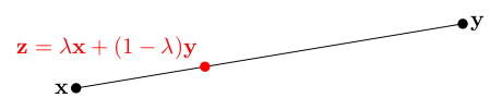
Given two points $x, y$ , a convex combination is any point $z$ that lies on the line between $x$ and $y$ . Algebraically, a convex combination is any point $z$ that can be represented as $z = λ x + (1 - λ) y$ for some multiplier $λ \in [0, 1]$ .

Schematic of a convex combination on a 2D plane: two black points x and y are joined by a line segment, with a red point z placed one-third of the way from y to x to illustrate z = lambda*x + (1-lambda)*y for lambda = 2/3. — Figure 6.1: A convex combination of the points $x$ and $y$ is given by $z = λ x + (1 - λ) y$ with any $λ \in [0, 1]$ . Here we demonstrate this using $λ = 2 ∕ 3$ .

Definition 6.8: Convex Set

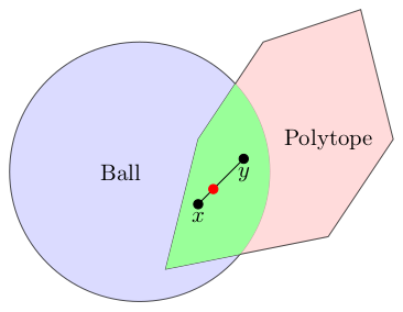
A set $C$ is convex if it contains all convex combinations of points in $C$ . That is, for any $x, y \in C$ , it holds that $λ x + (1 - λ) y \in C$ for all $λ \in [0, 1]$ .

(a) Convex Set

(b) Non-convex Set

Figure 6.2: A convex set and a non-convex set.

Some examples of convex sets are:

1.: Hyperplane $H = {x \in ℝ^{n} : a^{⊤} x = b}$
2.: Halfspace $H = {x \in ℝ^{n} : a^{⊤} x \leq b}$
3.: Polyhedron $P = {x \in ℝ^{n} : A x \leq b}$
4.: Ball $B = {x \in ℝ^{n} : \sum_{i = 1}^{n} x_{i}^{2} \leq 1}$
5.: Second Order Cone $S = {(x, t) \in ℝ^{n} \times ℝ : ∥ x ∥ \leq t}$ , i.e., $\sum_{i = 1}^{n} x_{i}^{2} \leq t^{2}$ with $t \geq 0$

Lemma 6.1. Intersection of Convex Sets is Convex Let $C_{1}$ and $C_{2}$ be convex sets. Then the intersection $C_{1} \cap C_{2}$ is convex. In particular,

C_{1} \cap C_{2} : = {x : x \in C_{1} and x \in C_{2}} .

The green intersection of the ball and the polytope, which is again a convex set. — Figure 6.4: The green intersection of the convex sets that are the ball and the polytope is also convex. This can be seen by considering any points $x, y \in Ball \cap Polytope$ . Since Ball is convex, the line segment between $x$ and $y$ is completely contained in Ball. And similarly, the line segment is completely contained in Polytope. Hence, the line segment is also contained in the intersection. This is how we can reason that the intersection is also convex.

Theorem 6.9: Convexity of Polyhedra

A polyhedron $P = {x \in ℝ^{n} : A x \leq b}$ , that is, the intersection of finitely many half-spaces, is a convex set.

Proof. Intuitively, convexity says that the line segment between any two points of the set stays inside the set. For a polyhedron defined by linear inequalities, this property follows directly from the linearity of those inequalities, as we now show.

Let $P$ be a polyhedron in $ℝ^{n}$ defined by the intersection of finitely many half-spaces:

P = {x \in ℝ^{n} : A x \leq b},

where $A$ is an $m \times n$ matrix, $x \in ℝ^{n}$ is a variable vector, and $b \in ℝ^{m}$ is a constant vector.

To prove $P$ is convex, we must show that for any two points $x_{1}, x_{2} \in P$ and any $λ \in [0, 1]$ , the convex combination

x_{λ} = λ x_{1} + (1 - λ) x_{2}

also lies in $P$ . In other words, we need to verify that $x_{λ}$ satisfies every constraint defining $P$ , namely $A x_{λ} \leq b$ .

Since $x_{1}, x_{2} \in P$ , each of them satisfies the defining inequalities:

A x_{1} \leq b and A x_{2} \leq b .

By linearity of matrix multiplication, we can distribute $A$ across the convex combination:

A x_{λ} = A (λ x_{1} + (1 - λ) x_{2}) = λ A x_{1} + (1 - λ) A x_{2} .

Because $λ \geq 0$ and $1 - λ \geq 0$ , multiplying the inequalities $A x_{1} \leq b$ and $A x_{2} \leq b$ by these non-negative scalars preserves their direction. Adding the two scaled inequalities together yields

λ A x_{1} + (1 - λ) A x_{2} \leq λ b + (1 - λ) b = b .

Combining the two displayed lines, we conclude that $A x_{λ} \leq b$ , so $x_{λ} \in P$ .

Since $x_{1}$ , $x_{2}$ , and $λ$ were arbitrary, every convex combination of points in $P$ remains in $P$ . Therefore $P$ is convex. □

Extreme Points: An extreme point of a polyhedral set $C$ is a point that cannot be written as a convex combination of other points in $C$ . Linear programming solutions often occur at extreme points, as guaranteed by fundamental theorems of linear programming.

Lemma 6.2. Objective Values on a Line Segment Given two points $x, y \in ℝ^{n}$ , a linear function evaluated at any point on the line segment between $x$ and $y$ is bounded above by the maximum of the evaluations at $x$ and $y$ . Formally, for any $c \in ℝ^{n}$ ,

\min {c^{⊤} x, c^{⊤} y} \leq c^{⊤} z \leq \max {c^{⊤} x, c^{⊤} y},

where $z = λ x + (1 - λ) y$ for some $λ \in (0, 1)$ .

Either both of these inequalities are strict, or they are both held at equality.

Proof. Expanding $c^{⊤} z$ based on the definition

\begin{array}{l} c^{⊤} z & = c^{⊤} (λ x + (1 - λ) y) & Replace formula for z \\ = c^{⊤} λ x + c^{⊤} (1 - λ) y & use distributivity \\ = λ c^{⊤} x + (1 - λ) c^{⊤} y & use linearity \end{array}

This equation expresses $c^{⊤} z$ as a convex combination of $c^{⊤} x$ and $c^{⊤} y$ . Since $λ \in [0, 1]$ , we know $λ \geq 0$ and $1 - λ \geq 0$ , ensuring that the combination is convex.

$One-dimensional number line showing c^T z between c^T x and c^T y. Three dots mark min and max of {c^T x, c^T y} and the convex combination c^T z = lambda c^T x + (1-lambda) c^T y in between.$

Figure 6.5: A number line showing that the objective value at z lies between the objective values at x and y.

By the properties of convex combinations, the value $c^{⊤} z$ lies between $c^{⊤} x$ and $c^{⊤} y$ . Formally:

\min {c^{⊤} x, c^{⊤} y} \leq c^{⊤} z \leq \max {c^{⊤} x, c^{⊤} y} .

Therefore, the value of $c^{⊤} z$ is bounded above by $\max {c^{⊤} x, c^{⊤} y}$ , as required. □

Theorem 6.10: Optimal Solution at an Extreme Point

Let $C \subseteq ℝ^{n}$ be a bounded, closed, and convex set. Let the objective be to maximize $c^{⊤} x$ over $C$ . Then, there exists an optimal solution $x^{*} \in C$ such that $x^{*}$ is an extreme point of $C$ .

Proof. Since $C$ is bounded and closed, it is compact in $ℝ^{n}$ . The linear function $c^{⊤} x$ is continuous, and by the Extreme Value Theorem, it attains its maximum value on the compact set $C$ . Let $x^{*} \in C$ be such that:

c^{⊤} x^{*} = \max {c^{⊤} x : x \in C}

Suppose $x^{*}$ is not an extreme point of $C$ . Then, $x^{*}$ can be expressed as a convex combination of two distinct points $x, y \in C$ :

x^{*} = λ x + (1 - λ) y, where λ \in (0, 1) .

By Lemma 6.2, the value $c^{⊤} x^{*}$ satisfies:

\min {c^{⊤} x, c^{⊤} y} \leq c^{⊤} x^{*} \leq \max {c^{⊤} x, c^{⊤} y} .

Since $x^{*}$ maximizes $c^{⊤} x$ over $C$ , it must be that $c^{⊤} x = c^{⊤} x^{*}$ and $c^{⊤} y = c^{⊤} x^{*}$ . Thus, both $x$ and $y$ also maximize $c^{⊤} x$ over $C$ .

If $x^{*}$ is not an extreme point, we can repeat this argument for $x$ and $y$ , expressing them as convex combinations of other points in $C$ . When $C$ is a polyhedron, this process must terminate after a finite number of steps because each step moves to a face of strictly smaller dimension and a polyhedron has only finitely many faces; at that point we reach an extreme point that maximizes $c^{⊤} x$ . (For a general compact convex set, termination requires a more careful argument, for instance induction on the dimension of $C$ ; we omit the details.)

Hence, there exists an optimal solution at an extreme point of $C$ . □

Theorem 6.11: Extreme Points and Vertices of a Polyhedron

Let $P \subseteq ℝ^{n}$ be a polyhedron. Then, a point $v \in P$ is an extreme point if and only if $v$ is a vertex of $P$ .

Proof. (If $v$ is not a vertex, then it is not an extreme point):

Suppose $v \in P$ is not a vertex. By definition, this means $v$ is not the unique solution to any subset of $n$ linearly independent constraints active at $v$ . Let $A^{'} x = b^{'}$ represent the active constraints at $v$ , where $A^{'} \in ℝ^{m^{'} \times n}$ ( $m^{'} \leq n$ ) is the matrix of active constraints, and assume the rows of $A^{'}$ are linearly independent. Since $v$ is not a vertex, the null space of $A^{'}$ , denoted $𝒩 (A^{'})$ , is nontrivial, i.e., there exists a nonzero direction $d \in ℝ^{n}$ such that:

A^{'} d = 0 .

Consider perturbing $v$ in the directions $v + 𝜖 d$ and $v - 𝜖 d$ , for some small $𝜖 > 0$ . Since $d \in 𝒩 (A^{'})$ , the perturbed points satisfy the active constraints:

A^{'} (v + 𝜖 d) = A^{'} v + 𝜖 A^{'} d = b^{'} .

Similarly, $A^{'} (v - 𝜖 d) = b^{'}$ .

For sufficiently small $𝜖 > 0$ , the perturbed points also satisfy all other constraints defining $P$ . This is because $P$ is a polyhedron, and the constraints are continuous linear inequalities that remain satisfied under small perturbations of $v$ .

Now, we express $v$ as a strict convex combination of $v + 𝜖 d$ and $v - 𝜖 d$ :

v = \frac{1}{2} (v + 𝜖 d) + \frac{1}{2} (v - 𝜖 d) .

Since $v + 𝜖 d \neq v$ and $v - 𝜖 d \neq v$ , and both points belong to $P$ , this shows that $v$ is not an extreme point of $P$ .

Figure 6.6: Two-dimensional plot of a quadrilateral polytope with vertices (0,0), (1,2), (3,2), (4,0).

(If $v$ is a vertex, then it is an extreme point):

Assume $v \in P$ is a vertex. By definition, there exists a subset of constraints, say $A^{'} x = b^{'}$ , where $A^{'} \in ℝ^{n \times n}$ , such that $v$ is the unique solution to this system.

Suppose, for the sake of contradiction, that $v$ is not an extreme point. Then, $v$ can be expressed as:

v = λ x_{1} + (1 - λ) x_{2}, x_{1}, x_{2} \in P, λ \in (0, 1),

where $x_{1} \neq v$ and $x_{2} \neq v$ .

We claim that both $x_{1}$ and $x_{2}$ must satisfy $A^{'} x = b^{'}$ . To see this, let $a$ be a row of $A^{'}$ and $b$ be the corresponding right hand side value in $b^{'}$ By Lemma 6.2, the value of $a^{⊤} v$ satisfies:

\min {a^{⊤} x_{1}, a^{⊤} x_{2}} \leq a^{⊤} v \leq \max {a^{⊤} x_{1}, a^{⊤} x_{2}} .

Since $v$ satisfies $a^{⊤} v = b$ , this implies:

a^{⊤} v = λ a^{⊤} x_{1} + (1 - λ) a^{⊤} x_{2} = b .

If either $a^{⊤} x_{1} \neq b$ or $a^{⊤} x_{2} \neq b$ , the equation above cannot hold. Hence, both $x_{1}$ and $x_{2}$ must satisfy $a^{⊤} x = b$ .

Since $v$ satisfies $A^{'} x = b^{'}$ , both $x_{1}$ and $x_{2}$ must also satisfy $A^{'} x = b^{'}$ , as $A^{'} x = b^{'}$ defines an affine subspace. However, this contradicts the assumption that $v$ is the unique solution to $A^{'} x = b^{'}$ .

Therefore, $v$ cannot be expressed as a strict convex combination of distinct points in $P$ , and $v$ is an extreme point.

Conclusion: A point $v \in P$ is an extreme point if and only if it is a vertex of $P$ . □

6.3.2 Unbounded Sets and Rays

Rays and Directions: A ray in $ℝ^{n}$ is a set of points:

{x : x = \bar{x} + λ d, λ \geq 0},

where $\bar{x}$ is the starting point and $d$ is the direction. Rays describe unbounded feasible regions in linear programming models.

Extreme Directions: An extreme direction is one that cannot be written as a positive combination of other directions. In linear programming, extreme directions help characterize unbounded solutions.

With these notions in hand, we can state a structural result: every point of a polyhedron $P$ can be built from the extreme points and extreme directions of $P$ .

Theorem 6.12: Representation Theorem

Let $P \subseteq ℝ^{n}$ be a nonempty polyhedron, let $x^{1}, x^{2}, \dots x^{k}$ be the set of extreme points of $P$ , and if $P$ is unbounded, $d^{1}, d^{2}, \dots d^{l}$ be the set of extreme directions. Then any $x \in P$ is equal to a convex combination of the extreme points and a non-negative linear combination of the extreme directions: $x = \sum_{j = 1}^{k} λ_{j} x^{j} + \sum_{j = 1}^{l} μ_{j} d^{j}$ , where $\sum_{j = 1}^{k} λ_{j} = 1$ , $λ_{j} \geq 0, \forall j = 1, 2, \dots, k$ , and $μ_{j} \geq 0, \forall j = 1, 2, \dots, l$ .

As an illustration, consider the LP below, whose feasible region $P$ is drawn on the right (in the $(x_{1}, x_{2})$ -plane, with the slack variables $s_{1}, s_{2}, s_{3}$ eliminated). This feasible region is unbounded, extending without limit to the upper right, which is why the theorem must allow for extreme directions. Its extreme points are $(0, 0)$ , $(0, 1)$ , and $(2, 3)$ , marked in the figure.

\begin{array}{l} \max & z = - 5 x_{1} - x_{2} \\ s.t. & x_{1} - 4 x_{2} + s_{1} = 0 \\ - x_{1} + x_{2} + s_{2} = 1 \\ - x_{1} + 2 x_{2} + s_{3} = 4 \\ x_{1}, x_{2}, s_{1}, s_{2}, s_{3} \geq 0 . \end{array}

Figure 6.7: Feasible region with the lines s1=0, s2=0, s3=0 marking where each slack variable vanishes; basic...

As a concrete use of the theorem, we represent the point $(1 ∕ 2, 1) \in P$ as a convex combination of the extreme points. Find $λ$ s to solve the following system of equations, subject to $λ_{1} + λ_{2} + λ_{3} = 1$ and $λ_{1}, λ_{2}, λ_{3} \geq 0$ :

λ_{1} [\begin{matrix} 0 \\ 0 \end{matrix}] + λ_{2} [\begin{matrix} 0 \\ 1 \end{matrix}] + λ_{3} [\begin{matrix} 2 \\ 3 \end{matrix}] = [\begin{matrix} 1 ∕ 2 \\ 1 \end{matrix}]

One solution is $λ_{1} = 1 ∕ 2$ , $λ_{2} = 1 ∕ 4$ , $λ_{3} = 1 ∕ 4$ : the weights are non-negative and sum to $1$ , so $(1 ∕ 2, 1)$ is a convex combination of the extreme points. Here no extreme directions are needed (all $μ_{j} = 0$ ); they would be required only for points outside the convex hull of the extreme points, farther out in the unbounded part of $P$ .

6.4 Exercises

Warm-ups

Exercise 6.13: Vector Operations

$⋆$ Let $v = [3, - 2, 4]$ and $u = [- 1, 0, 2]$ . Compute:

1.: $v + u$
2.: $2 v$
3.: $v \cdot u$

[§6.1]

Exercise 6.14: Linear and Convex Combinations

$⋆$ Let $v^{1} = [1, 0]$ , $v^{2} = [0, 1]$ , and $v^{3} = [1, 1]$ .

1.

Which of the following are linear combinations of

v^{1}

and

v^{2}

$[2, 3]$
$[1, 1]$
$[1, - 1]$

2.

Is the vector

[1 ∕ 2, 1 ∕ 2]

a convex combination of any two of these vectors?

[§6.1, §6.3]

Exercise 6.15: Linear Independence and Matrix Rank

$⋆$ Consider the matrix $A = [\begin{matrix} 1 & 2 \\ 2 & 4 \end{matrix}]$ .

1.: Are the rows of $A$ linearly independent?
2.: Are the columns linearly independent?
3.: What is $rank (A)$ ?

[§6.1]

Exercise 6.16: Convex or Not?

$⋆$ For each of the following subsets of $ℝ^{2}$ , decide whether the set is convex, as in Figures 6.2a and 6.2b. If the set is not convex, exhibit two points in the set whose connecting segment leaves the set.

1.: The disk $D = {x : x_{1}^{2} + x_{2}^{2} \leq 4}$ .
2.: The ring $R = {x : 1 \leq x_{1}^{2} + x_{2}^{2} \leq 4}$ .
3.: The halfspace $H = {x : x_{1} + 2 x_{2} \leq 3}$ .
4.: The set $S = {x : | x_{1} | \geq 1}$ .

[§6.3]

Exercise 6.17: Writing an LP in Matrix Notation

$⋆$ Consider the linear program

\begin{array}{l} \max & 3 x_{1} + 2 x_{2} \\ s.t. & x_{1} + 3 x_{2} \leq 6 \\ 2 x_{1} + x_{2} \leq 4 \\ x_{1}, x_{2} \geq 0 . \end{array}

Write this LP in the standard form $\max {c^{⊤} x : A x \leq b}$ used in this chapter: give the vector $c$ , the $4 \times 2$ matrix $A$ , and the vector $b$ . (Write each nonnegativity constraint $x_{i} \geq 0$ as $- x_{i} \leq 0$ .) Then verify that the point $x = (1.2, 1.6)$ satisfies $A x \leq b$ .

[§6.1, §6.2]

Core problems

Exercise 6.18: Convex Combinations and Geometry

$⋆ ⋆$ Let $P$ be the triangle with vertices at $(0, 0)$ , $(2, 0)$ , and $(0, 2)$ .

1.: Plot the set $P$ .
2.: Determine whether the point $(1, 1)$ is a convex combination of the vertices.
3.: Determine whether the point $(1.5, 1.5)$ is in $P$ .

[§6.3]

Exercise 6.19: Halfspace Geometry and Convexity

$⋆ ⋆$ Consider the halfspace $H = {x \in ℝ^{2} : x_{1} + 2 x_{2} \leq 4}$ .

1.: Plot the halfspace and the boundary.
2.: Is the point $(2, 1)$ in $H$ ? What about $(1, 2)$ ?
3.: Verify that the set is convex by checking whether the midpoint between $(0, 0)$ and $(2, 1)$ lies in $H$ .

[§6.3, Theorem 6.9]

Exercise 6.20: Checking an Extreme Point

$⋆ ⋆$ Let

P = {x \in ℝ^{2} : x_{1} - 4 x_{2} \leq 0, - x_{1} + x_{2} \leq 1, - x_{1} + 2 x_{2} \leq 4, x_{1} \geq 0, x_{2} \geq 0}

be the feasible region used to illustrate the Representation Theorem.

1.: Verify that $(2, 3) \in P$ , identify the constraints that are tight there, and show that the tight rows are linearly independent. Conclude that $(2, 3)$ is a vertex of $P$ , and hence an extreme point.
2.: Verify that $(1, 2) \in P$ and show that only one constraint is tight there. Then express $(1, 2)$ as a convex combination of two other points of $P$ to conclude that $(1, 2)$ is not an extreme point.

[§6.2, §6.3]

Exercise 6.21: A Convex Combination of Extreme Points

$⋆ ⋆$ The polyhedron $P$ from Exercise 6.20 has extreme points $(0, 0)$ , $(0, 1)$ , and $(2, 3)$ . Following the illustration of the Representation Theorem, find multipliers $λ_{1}, λ_{2}, λ_{3} \geq 0$ with $λ_{1} + λ_{2} + λ_{3} = 1$ such that

λ_{1} [\begin{matrix} 0 \\ 0 \end{matrix}] + λ_{2} [\begin{matrix} 0 \\ 1 \end{matrix}] + λ_{3} [\begin{matrix} 2 \\ 3 \end{matrix}] = [\begin{matrix} 1 \\ 7 ∕ 4 \end{matrix}] .

Why are no extreme directions needed to represent this point?

[§6.3, Theorem 6.12]

Concepts and connections

Exercise 6.22: Is the Union of Convex Sets Convex?

$⋆ ⋆$ The chapter shows that the intersection of two convex sets is always convex.

1.: Give an example of two convex sets $C_{1}, C_{2} \subseteq ℝ^{2}$ whose union $C_{1} \cup C_{2}$ is not convex, and verify your claim by exhibiting two points of the union whose midpoint is not in the union.
2.: Find a condition on $C_{1}$ and $C_{2}$ under which the union is convex, and justify it.

[§6.3]

Exercise 6.23: Where Boundedness Enters the Vertex Theorem

$⋆ ⋆$ The proof in §6.2 that some optimal solution lies at a vertex assumes the feasible region $P$ is bounded.

1.: Point to the exact step of the proof where boundedness is used, and explain what could go wrong without it.
2.: Let $P = {x \in ℝ^{2} : 0 \leq x_{2} \leq 1}$ and consider maximizing $- x_{2}$ over $P$ . Show that $P$ has no vertex at all, that the LP nevertheless has optimal solutions, and describe the set of optima. Which hypothesis of the theorem fails, and why does this example not contradict the theorem?

[§6.2]

Challenge problems

Exercise 6.24: Intersections of Arbitrary Families of Convex Sets

$⋆ ⋆ ⋆$ Let ${C_{i}}_{i \in I}$ be any family of convex sets in $ℝ^{n}$ , where the index set $I$ may be infinite. Prove that the intersection

C = ⋂_{i \in I} C_{i}

is convex. Explain why this result, applied to halfspaces, gives another proof of Theorem 6.9. (Note that $C$ may be empty; the empty set is convex vacuously.)

[§6.3, Theorem 6.9]

Selected Solutions

Solution

(Exercise 6.13) Working componentwise:

1.: $v + u = [3 + (- 1), - 2 + 0, 4 + 2] = [2, - 2, 6]$ .
2.: $2 v = [6, - 4, 8]$ .
3.: $v \cdot u = (3) (- 1) + (- 2) (0) + (4) (2) = - 3 + 0 + 8 = 5$ .

Solution

(Exercise 6.18) The triangle $P$ is the set of convex combinations of $(0, 0)$ , $(2, 0)$ , and $(0, 2)$ ; equivalently, $P = {x \in ℝ^{2} : x_{1} \geq 0, x_{2} \geq 0, x_{1} + x_{2} \leq 2}$ .

1.

The plot is the triangle with the three given vertices.

2.

Yes. Take

λ_{1} = 0

λ_{2} = λ_{3} = \frac{1}{2}

0 [\begin{matrix} 0 \\ 0 \end{matrix}] + \frac{1}{2} [\begin{matrix} 2 \\ 0 \end{matrix}] + \frac{1}{2} [\begin{matrix} 0 \\ 2 \end{matrix}] = [\begin{matrix} 1 \\ 1 \end{matrix}],

and the weights are nonnegative and sum to $1$ .

3.

No. Any combination of the vertices hitting

(1.5, 1.5)

must satisfy

2 λ_{2} = 1.5

and

2 λ_{3} = 1.5

, forcing

λ_{2} = λ_{3} = 0.75

and

λ_{2} + λ_{3} = 1.5 > 1

. Equivalently,

1.5 + 1.5 = 3 > 2

violates

x_{1} + x_{2} \leq 2

, so

(1.5, 1.5) \notin P

Solution

(Exercise 6.21) The first coordinate forces $2 λ_{3} = 1$ , so $λ_{3} = 1 ∕ 2$ . The second coordinate then gives $λ_{2} + 3 ∕ 2 = 7 ∕ 4$ , so $λ_{2} = 1 ∕ 4$ , and the normalization $λ_{1} + λ_{2} + λ_{3} = 1$ gives $λ_{1} = 1 ∕ 4$ . All three multipliers are nonnegative, so

\frac{1}{4} [\begin{matrix} 0 \\ 0 \end{matrix}] + \frac{1}{4} [\begin{matrix} 0 \\ 1 \end{matrix}] + \frac{1}{2} [\begin{matrix} 2 \\ 3 \end{matrix}] = [\begin{matrix} 1 \\ 7 ∕ 4 \end{matrix}],

and $(1, 7 ∕ 4)$ is a convex combination of the extreme points. No extreme directions are needed because $(1, 7 ∕ 4)$ already lies in the convex hull of the three extreme points; all coefficients $μ_{j}$ in the Representation Theorem can be taken to be zero.

Solution

(Exercise 6.22)

1.: Take $C_{1}$ to be the unit disk centered at $(- 2, 0)$ and $C_{2}$ the unit disk centered at $(2, 0)$ . Each disk is convex. The points $(- 2, 0) \in C_{1}$ and $(2, 0) \in C_{2}$ both lie in the union, but their midpoint $(0, 0)$ is at distance $2 > 1$ from both centers, so it lies in neither disk. Hence $C_{1} \cup C_{2}$ is not convex.
2.: If one set contains the other, say $C_{1} \subseteq C_{2}$ , then $C_{1} \cup C_{2} = C_{2}$ , which is convex. Nesting is sufficient but not necessary: with $C_{1} = {x : x_{2} \geq 0}$ and $C_{2} = {x : x_{2} \leq 0}$ , neither halfplane contains the other, yet $C_{1} \cup C_{2} = ℝ^{2}$ is convex.

Chapter 6Formal Mathematical Statements

6.1 Mathematical Preliminaries

6.1.1 Vectors and Their Properties

6.1.2 Linear Combinations and Related Concepts

6.2 Algebraic Proof - Exists Optimal Solution at a Vertex

6.3 Convexity

6.3.1 Convex Sets

6.3.2 Unbounded Sets and Rays

6.4 Exercises

Selected Solutions

Chapter 6
Formal Mathematical Statements