5 Graphically Solving Linear Programs

Contents | ‹ Previous | Next › | Download EPUB | PDF

Chapter 5
Graphically Solving Linear Programs

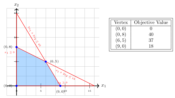
Learning Outcomes

A.: Draw the region of points allowed by the constraints, together with level lines of the objective.
B.: Locate the corner points of that region and compute their coordinates.
C.: Read an optimal solution directly off the picture.
D.: Recognize the four ways a linear program can turn out: a single best point, a whole edge of best points, no allowed points at all, or an objective that grows without limit.

Resources

Try it out visually!

Objective-Level Slider: drag the objective line across the feasible region and watch where optima land.

A linear program with two decision variables fits entirely on a sheet of paper: each constraint cuts the plane with a line, the points surviving every cut form the feasible region, and the objective becomes a family of parallel lines, one for each possible objective value. Sliding a line from this family across the region and watching where it exits gives a purely visual way to locate a best possible point, and this picture is the subject of the present chapter.

Our starting point is a small, well-behaved example whose picture is easy to draw. Once its geometry is understood, we move on to examples where things go wrong in instructive ways.

5.1 Nonempty and Bounded Problem

Consider the problem

\begin{array}{l} \max & 2 x_{1} + 5 x_{2} \\ s.t. & x_{1} + 2 x_{2} \leq 16 \\ 5 x_{1} + 3 x_{2} \leq 45 \\ x_{1}, x_{2} \geq 0 \end{array}

The first step is a picture of the feasible region: every point $(x_{1}, x_{2})$ that survives all of the constraints at once.

A reliable way to draw it is boundary-first: sketch the line where each constraint holds with equality, namely

$x_{1} + 2 x_{2} = 16$
$5 x_{1} + 3 x_{2} = 45$
$x_{1} = 0$
$x_{2} = 0$

and then shading in the side of the space cut out by the corresponding inequality.

Two-dimensional plot of the feasible region for max 2x_1+5x_2 with vertices (0,0), (9,0), (6,5), (0,8), bounded by x_1+2x_2<=16 and 5x_1+3x_2<=45 (red); an inset table lists the objective value at each vertex (0, 18, 37, 40). — Figure 5.1: Desmos: Interactive plot! (backup interactive plot)

Each line splits the plane in two; keeping the correct side of every line and shading whatever survives produces the feasible region.

Two features of this particular region are worth naming. It is nonempty: at least one point satisfies every constraint. And it is bounded: the whole region fits inside some large circle, with no direction in which it stretches forever.

The corners of the region, called extreme points, will turn out to carry all the information we need about optimal solutions. Each corner sits where two of the boundary lines cross, so corner coordinates come from solving $2 \times 2$ linear systems. Watch out, though: crossing two boundary lines is necessary but not sufficient, since two lines can also intersect at a point that violates some third constraint.

We will later use the terminology basic feasible solution for an extreme point of the feasible region, and basic solution as a point that is the intersection of 2 lines, but is actually infeasible (does not satisfy all the constraints).

Theorem 5.1: Optimal Solution at a Vertex

If the feasible region of the linear program is nonempty and bounded, then there exists an optimal solution at a vertex of the feasible region.

This theorem implies the following algorithm.

Algorithm: Enumerate Vertices Algorithm for Solving a Linear Programming Problem

1.: Identify the Feasible Region: Determine the set of constraints defining the feasible region in the problem.
2.: Enumerate Vertices: Find all the vertices (corner points) of the feasible region. This can be done by solving pairs of constraint equations to find their intersections, keeping only those that satisfy all constraints.
3.: Compute Objective Values: Evaluate the objective function at each vertex of the feasible region.
4.: Compare Objective Values: For a maximization problem, identify the vertex with the highest objective value. For a minimization problem, identify the vertex with the lowest objective value.
5.: Determine the Optimal Solution: The vertex with the optimal objective value is the solution to the linear programming problem.

We will explore why Theorem 5.1 is true, and also what happens when the feasible region does not satisfy the assumptions of either nonempty or bounded.

5.2 Graphical Approach

We now apply the vertex enumeration idea graphically using a concrete example.

Example 5.2: Furniture Workshop

A small furniture workshop produces chairs and tables. Each chair requires 2 hours of carpentry and 1 hour of finishing, earning a profit of $8. Each table requires 1 hour of carpentry and 3 hours of finishing, earning a profit of $6. The workshop has 80 hours of carpentry time and 90 hours of finishing time available per week. Market demand limits chair production to at most 32 per week.

Letting $x_{1}$ denote the number of chairs and $x_{2}$ the number of tables, the linear program is:

\begin{aligned} max & z(x_{1}, x_{2}) = 8 x_{1} + 6 x_{2} \\ s.t. & 2 x_{1} + x_{2} ≤ 80 \\ x_{1} + 3 x_{2} ≤ 90 \\ x_{1} ≤ 32 \\ x_{1} ≥ 0 \\ x_{2} ≥ 0 \end{aligned}

(5.1)

Solution

To solve graphically, we first sketch the feasible region by plotting the boundary lines of each constraint and shading the region that satisfies all inequalities simultaneously. The result is shown in Figure 5.2.

Graphical method plot on x1-x2 axes running to about 90: red constraint lines bound a shaded feasible region with blue corner points labeled (0,30), (30,20), and (35,10); gray dashed level lines of the objective sweep across the region toward the optimal vertex. — Figure 5.2: Feasible region and level curves for the Furniture Workshop problem. The shaded polygon represents the set of all $(x_{1}, x_{2})$ satisfying every constraint. Dashed lines show the objective function at several values of $z$ . As $z$ increases, the level curves sweep upward and to the right.

Next, we overlay level curves of the objective function. Setting $8 x_{1} + 6 x_{2} = z$ gives the family of lines

x_{2} = - \frac{4}{3} x_{1} + \frac{z}{6},

which are parallel lines with slope $- 4 ∕ 3$ . Increasing $z$ shifts them in the direction of the gradient $\nabla z = (8, 6)$ . Sweeping the level curves in this direction, the last one to touch the feasible region does so at the vertex $(x_{1}^{*}, x_{2}^{*}) = (30, 20)$ , yielding the optimal profit

z^{*} = 8 (30) + 6 (20) = 360 .

This optimal point sits at the intersection of the two constraints $2 x_{1} + x_{2} = 80$ and $x_{1} + 3 x_{2} = 90$ . Both constraints are satisfied with equality at the optimum; we say they are binding. The remaining constraints ( $x_{1} \leq 35$ , $x_{1} \geq 0$ , $x_{2} \geq 0$ ) are satisfied strictly and are non-binding.

This illustrates a general principle: when an optimal solution to a linear program exists, it occurs at a vertex of the feasible region, the intersection of several binding constraints.

We can now state a preliminary algorithm for solving a two-variable LP with a bounded feasible region graphically.

➀ Graphical Method 1: Bounded Region, Unique Optimum

1.: Sketch the feasible region by plotting each constraint boundary and shading the intersection of all half-planes.
2.: Draw several level curves of the objective function $z = c_{1} x_{1} + c_{2} x_{2}$ for increasing values of $z$ .
3.: Sweep the level curves in the gradient direction $\nabla z = (c_{1}, c_{2})$ until the last level curve that still touches the feasible region is found.
4.: The vertex of the feasible region lying on this last level curve is the optimal solution.

Example 5.3: Lemonade Vendor

Say you are a vendor of lemonade and lemon juice. Each unit of lemonade requires 1 lemon and 2 litres of water. Each unit of lemon juice requires 3 lemons and 1 litre of water. Each unit of lemonade gives a profit of three dollars. Each unit of lemon juice gives a profit of two dollars. You have 6 lemons and 4 litres of water available. How many units of lemonade and lemon juice should you make to maximize profit?

If we let $x$ denote the number of units of lemonade to be made and let $y$ denote the number of units of lemon juice to be made, then the profit is given by $3 x + 2 y$ dollars. We call $3 x + 2 y$ the objective function. Note that there are a number of constraints that $x$ and $y$ must satisfy. First of all, $x$ and $y$ should be nonnegative. The number of lemons needed to make $x$ units of lemonade and $y$ units of lemon juice is $x + 3 y$ and cannot exceed 6. The number of litres of water needed to make $x$ units of lemonade and $y$ units of lemon juice is $2 x + y$ and cannot exceed 4. Hence, to determine the maximum profit, we need to maximize $3 x + 2 y$ subject to $x$ and $y$ satisfying the constraints $x + 3 y \leq 6$ , $2 x + y \leq 4$ , $x \geq 0$ , and $y \geq 0 .$

A more compact way to write the problem is as follows:

\begin{matrix} maximize & 3 x & + & 2 y \\ subject to & x & + & 3 y & \leq & 6 \\ 2 x & + & y & \leq & 4 \\ x & \geq & 0 \\ y & \geq & 0 . \end{matrix}

Solution

We can solve this maximization problem graphically as follows. We first sketch the set of $(x, y)$ satisfying the constraints, called the feasible region, on the $(x, y)$ -plane. We then take the objective function $3 x + 2 y$ and turn it into an equation of a line $3 x + 2 y = z$ where $z$ is a parameter. Note that as the value of $z$ increases, the line defined by the equation $3 x + 2 y = z$ moves in the direction of the normal vector $(3, 2)$ . We call this direction the direction of improvement. Determining the maximum value of the objective function, called the optimal value, subject to the constraints amounts to finding the maximum value of $z$ so that the line defined by the equation $3 x + 2 y = z$ still intersects the feasible region.

Feasible region plot on x-y axes: blue shaded polygon bounded by red constraint lines 2x + y = 4 and x + 3y = 6 and the axes, with the optimal vertex labeled (1.2, 1.6); dashed gray objective level lines increase toward that vertex. — Figure 5.3: Feasible region and objective level curves for the Lemonade Vendor problem. The shaded polygon is the set of $(x, y)$ satisfying all constraints; dashed lines are level curves $3 x + 2 y = z$ for $z = 0, 2, 4, 6, 8$ . Sweeping the level curves in the direction of $\nabla z = (3, 2)$ shows the optimum is at the vertex $(1.2, 1.6)$ .

Blue shaded triangular feasible region on x1-x2 axes bounded by three lines labeled -x1 + 2x2 <= 3, x1 + 2x2 >= 3, and 2x1 + x2 <= 5. — Figure 5.4: Feasible region of a generic linear program with constraints $x_{1} + x_{2} \geq 3$ , $2 x_{1} - x_{2} \leq 5$ , and $- x_{1} + 2 x_{2} \leq 3$ . The shaded triangle illustrates how three linear inequalities can carve out a bounded polygonal region.

In Figure 5.3, level curves of $z = 3 x + 2 y$ are drawn for several values of $z$ . From the picture, we can see that if $z$ is greater than 6.8, the line defined by $3 x + 2 y = z$ will not intersect the feasible region. Hence, the profit cannot exceed 6.8 dollars.

As the line $3 x + 2 y = 6.8$ does intersect the feasible region, $6.8$ is the maximum value for the objective function. Note that there is only one point in the feasible region that intersects the line $3 x + 2 y = 6.8$ , namely $(x, y) = (1.2, 1.6)$ . In other words, to maximize profit, we want to make 1.2 units of lemonade and 1.6 units of lemon juice.

The examples above each have a single optimal solution. However, four qualitatively different outcomes are possible for any linear program:

1.: A unique optimal solution (as we have already seen).
2.: Infinitely many optimal solutions (the optimal level curve is parallel to an edge of the feasible region).
3.: The problem is unbounded: the objective value can be made arbitrarily large (maximization) or small (minimization).
4.: The problem is infeasible: no point satisfies all constraints simultaneously.

The third outcome can only arise when the feasible region is unbounded. We will illustrate each of these outcomes below and, in a later chapter, prove that these are the only possibilities.

5.3 Infinitely Many Optimal Solutions

It is possible for a linear program to have more than one optimal solution. When this happens, there are in fact infinitely many. We illustrate with a modification of the Furniture Workshop.

Example 5.4: Furniture Workshop: Alternative Objective

Suppose the workshop in Example 5.2 revises its pricing so that each chair earns $2 and each table earns $1. The new objective function is $z (x_{1}, x_{2}) = 2 x_{1} + x_{2}$ , while the constraints remain unchanged:

\begin{aligned} max & z(x_{1}, x_{2}) = 2 x_{1} + x_{2} \\ s.t. & 2 x_{1} + x_{2} ≤ 80 \\ x_{1} + 3 x_{2} ≤ 90 \\ x_{1} ≤ 35 \\ x_{1}, x_{2} ≥ 0 \end{aligned}

(5.2)

Solution

The gradient of the new objective is $\nabla z = (2, 1)$ , which is parallel to the constraint $2 x_{1} + x_{2} = 80$ . As we sweep the level curves in the gradient direction, the last level curve that touches the feasible region coincides with the entire edge from $(30, 20)$ to $(35, 10)$ . Along this edge, $2 x_{1} + x_{2} = 80$ for every point, so $z = 80$ everywhere on it.

Graphical method plot: shaded feasible region with blue corner points (0,30), (30,20), and (35,10); gray dashed objective level lines labeled z = 20, 40, 60, 80 sweep the region, showing the optimum at a corner. — Figure 5.5: Alternative optimal solutions: the level curve $z = 80$ (bold blue segment) lies along an entire edge of the feasible region. Every point on this edge is an optimal solution.

Let $P$ denote the feasible region. For any $x_{1}^{*} \in [30, 35]$ with $x_{2}^{*} = 80 - 2 x_{1}^{*}$ , the point $(x_{1}^{*}, x_{2}^{*})$ lies on the edge from $(30, 20)$ to $(35, 10)$ , and $z (x_{1}^{*}, x_{2}^{*}) = 80 \geq z (x_{1}, x_{2})$ for all $(x_{1}, x_{2}) \in P$ . Since there are infinitely many such points, the problem has infinitely many optimal solutions.

Based on this example, we extend our graphical algorithm to handle multiple optimal solutions:

➁ Graphical Method 2: Allowing Multiple Optima

Everything from Method 1, plus a check for ties.

1.: Sketch the feasible region by plotting each constraint boundary.
2.: Draw level curves of the objective function for several values of $z$ .
3.: Sweep the level curves in the gradient direction to find the optimal value of $z$ that still intersects the feasible region. An optimal solution will occur at a vertex.
4.: If the optimal level curve is parallel to an edge of the feasible region adjacent to the optimal vertex, then every point on that edge is also optimal. The problem has infinitely many optimal solutions.

Learning Checkpoint 5.3.1

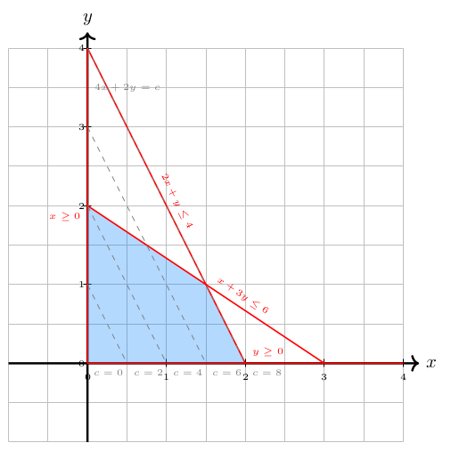
Consider the graphical representation below. How many optimal solutions are there if we are maximizing? How about if we are minimizing?

5.4 Problems with No Solution

When the constraints of a linear program contradict one another, no point can satisfy them all. The feasible region is empty and we say the problem is infeasible.

Example 5.5: Infeasible Problem

Consider the following linear programming problem:

\begin{aligned} max & z(x_{1}, x_{2}) = 4 x_{1} + 3 x_{2} \\ s.t. & x_{1} + x_{2} ≤ 8 \\ 2 x_{1} + x_{2} ≤ 12 \\ x_{1} ≥ 7 \\ x_{2} ≥ 5 \end{aligned}

(5.3)

Solution

The constraints are plotted in Figure 5.6. The first two constraints restrict $x_{1} + x_{2} \leq 8$ , but the lower bounds $x_{1} \geq 7$ and $x_{2} \geq 5$ together require $x_{1} + x_{2} \geq 12$ . These are contradictory, so no point satisfies all constraints simultaneously.

Infeasible LP illustration: constraint boundaries 2x1 + x2 <= 12 (blue) and x1 + x2 <= 8 (red) shade toward the origin while x2 >= 5 (orange) and x1 >= 7 (green) shade away from it; the note 'No feasible region' marks the empty intersection. — Figure 5.6: An infeasible linear program. The upper-bound constraints force $x_{1} + x_{2} \leq 8$ , but the lower bounds require $x_{1} \geq 7$ and $x_{2} \geq 5$ , so $x_{1} + x_{2} \geq 12$ . No point can satisfy both conditions, and the feasible region is empty.

Since the feasible region is empty, the problem has no solution.

Before stating the complete graphical algorithm, we also consider the case of unbounded feasible regions.

5.5 Problems with Unbounded Feasible Regions

Consider the problem

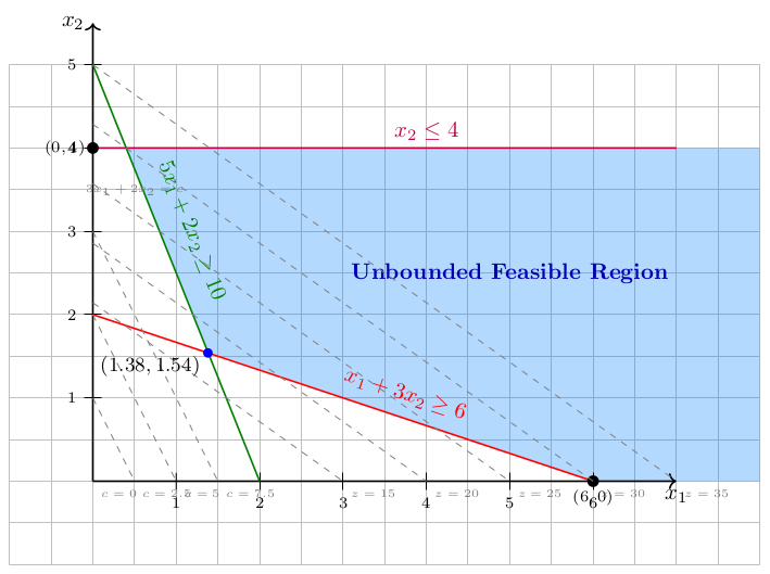
\begin{array}{l} \min & z = 5 x_{1} + 7 x_{2} \\ s.t. & x_{1} + 3 x_{2} & \geq 6 \\ 5 x_{1} + 2 x_{2} & \geq 10 \\ x_{2} & \leq 4 \\ x_{1}, x_{2} & \geq 0 \end{array}

As you can see, the feasible region is unbounded. In particular, from any point in the feasible region, one can always find another feasible point by increasing the $x_{1}$ coordinate (i.e., move to the right in the picture). However, this does not necessarily mean that the optimization problem is unbounded.

Indeed, the optimal solution is at $x^{*} = (1.38, 1.54)$ , the extreme point in the lower left hand corner, with optimal objective value

z^{*} = 5 \cdot 1.38 + 7 \cdot 1.54 = 17.7 .

Consider however, if we consider a different problem where we try to maximize the objective

\begin{array}{l} \max & z = 5 x_{1} + 7 x_{2} \\ s.t. & x_{1} + 3 x_{2} & \geq 6 \\ 5 x_{1} + 2 x_{2} & \geq 10 \\ x_{2} & \leq 4 \\ x_{1}, x_{2} & \geq 0 \end{array}

Solution

This optimization problem is unbounded! For example, notice that the point $(x_{1}, x_{2}) = (n, 0)$ is feasible for all $n = 1, 2, 3, \dots$ . Then the objective function $z = 5 n + 0$ follows the sequence $5, 10, 15, \dots$ , which diverges to infinity.

We now illustrate two more scenarios with unbounded feasible regions. In the first, the problem is unbounded; in the second, a finite optimum exists despite the unbounded region.

Example 5.6: Unbounded Problem

Consider the linear programming problem:

\begin{aligned} max & z(x_{1}, x_{2}) = x_{1} + 3 x_{2} \\ s.t. & x_{1} − x_{2} ≤ 3 \\ x_{1} + 2 x_{2} ≥ 4 \\ x_{1}, x_{2} ≥ 0 \end{aligned}

(5.4)

Solution

The feasible region and level curves are shown in Figure 5.7.

Unbounded feasible region: blue shaded area above two red constraint boundaries meeting at labeled corner points (0,2) and (3,1); gray dashed level lines of the objective x1 + 3x2 = z increase into the unbounded region, so the LP is unbounded. — Figure 5.7: An unbounded linear program. The feasible region extends infinitely upward and to the right. Level curves of $z = x_{1} + 3 x_{2}$ continue to intersect the feasible region for arbitrarily large $z$ , so the problem is unbounded.

The feasible region extends infinitely upward and to the right. For any target value $z_{0}$ , we can find a feasible point achieving $z \geq z_{0}$ . For instance, take $(x_{1}, x_{2}) = (0, t)$ for $t \geq 2$ : then $0 - t = - t \leq 3$ and $0 + 2 t = 2 t \geq 4$ , so the point is feasible, and $z = 3 t$ , which grows without bound. Hence the optimal value is $+ \infty$ and the problem is unbounded.

An unbounded feasible region does not always lead to an unbounded objective. The key is whether the gradient of the objective points into the unbounded direction or away from it.

Example 5.7: Finite Optimum with Unbounded Feasible Region

Consider the same feasible region as in Example 5.6 but with a new objective:

\begin{aligned} min & z(x_{1}, x_{2}) = 3 x_{1} + x_{2} \\ s.t. & x_{1} − x_{2} ≤ 3 \\ x_{1} + 2 x_{2} ≥ 4 \\ x_{1}, x_{2} ≥ 0 \end{aligned}

(5.5)

Solution

The feasible region is the same unbounded region as before. However, we are now minimizing, and the gradient $(3, 1)$ points to the right and slightly upward, precisely into the unbounded part of the feasible region. Moving opposite to the gradient (toward smaller $z$ ) takes us to the lower-left corner of the feasible region.

The same unbounded feasible region with a different objective: dashed level lines of 3x1 + x2 = z now achieve their minimum at a corner point, showing that an LP over an unbounded region can still have a finite optimum. Corner points (0,2) and (3,1) are marked. — Figure 5.8: A linear program with an unbounded feasible region but a finite optimal solution. The minimum of $z = 3 x_{1} + x_{2}$ occurs at the vertex $(0, 2)$ with $z^{*} = 2$ , because the gradient points away from the bounded end of the feasible region.

Evaluating the objective at the vertices: $z (0, 2) = 2$ and $z (\frac{10}{3}, \frac{1}{3}) = 10 + \frac{1}{3} = \frac{31}{3} \approx 10.3$ . Since we are minimizing, the optimum is $z^{*} = 2$ at $(x_{1}^{*}, x_{2}^{*}) = (0, 2)$ . Once again, the optimal solution occurs at a vertex of the feasible region, even though the region is unbounded.

We can now state a complete algorithm for graphically solving any two-variable linear program.

✓ The Complete Graphical Method for Two-Variable LPs

Handles every case: infeasible, unbounded, unique, and multiple optima.

1.

Sketch the feasible region by plotting the constraint boundaries and shading their intersection.

2.

If the feasible region is empty, the problem is infeasible; stop.

3.

Draw level curves of the objective function and determine the gradient direction.

4.

Bounded feasible region:

(a): Sweep the level curves in the gradient direction (for maximization) or opposite (for minimization) to find the last level curve touching the feasible region. The optimal solution is at a vertex.
(b): If this optimal level curve is parallel to an edge of the feasible region, every point on that edge is optimal (infinitely many solutions).

5.

Unbounded feasible region:

(a): If the level curves can be swept indefinitely while still intersecting the feasible region, the problem is unbounded.
(b): Otherwise, a finite optimum exists at a vertex; proceed as in the bounded case.

5.6 Exercises

Warm-ups

Exercise 5.8: Feasible Region Analysis

$⋆$ Consider the following system of constraints:

x + y \geq 5

x \geq 0, y \geq 0

Which of the following statements is true about the feasible region?

1.: The feasible region is a bounded polygon.
2.: The feasible region is an unbounded region.
3.: The feasible region consists of a single point.
4.: The problem is infeasible.

[§5.1, §5.5]

Exercise 5.9: Sketch Feasible Region

$⋆$ Sketch all $[\begin{matrix} x \\ y \end{matrix}]$ satisfying

x - 2 y \leq 2

on the $(x, y)$ -plane.

[§5.1]

Exercise 5.10: Graphical Method 1 Practice

$⋆$ Apply the steps of the box “Graphical Method 1: Bounded Region, Unique Optimum” to the linear program

\begin{array}{l} \max & 3 x + 2 y \\ s.t. & x + y \leq 4 \\ x \leq 3 \\ x, y \geq 0 . \end{array}

Sketch the feasible region, list all four vertices, and sweep the level curves of $z = 3 x + 2 y$ in the gradient direction to find the optimal solution and the optimal value.

[§5.2, Example 5.2]

Exercise 5.11: Graphical Method for Lemonade Vendor

$⋆$ Solve the Lemonade Vendor problem from Example 5.3 using the graphical method.

[§5.2, Example 5.3]

Core problems

Exercise 5.12: Graphical Method

$⋆ ⋆$ Use the graphical method to determine two optimal solutions to linear program:

\begin{array}{l} \min & 3 x_{1} + 5 x_{2} \\ 3 x_{1} + 2 x_{2} \geq 36 \\ 6 x_{1} + 10 x_{2} \geq 90 \\ x_{1}, x_{2} \geq 0 \end{array}

[§5.3, Example 5.4]

Exercise 5.13: Infeasible Region Graph

$⋆ ⋆$ Graph the feasible region of the linear program:

\begin{array}{l} \min & x_{1} - x_{2} \\ x_{1} + x_{2} \leq 6 \\ x_{1} - x_{2} \geq 1 \\ x_{2} - x_{1} \geq 3 \\ x_{1}, x_{2} \geq 0 \end{array}

Without considering the objective function, how many feasible solutions are there? Justify your answer.

[§5.4, Example 5.5]

Exercise 5.14: Determine Optimal Value

$⋆ ⋆$ Determine the optimal value of

\begin{matrix} Minimize & x + y \\ Subject to & 2 x + y \geq 4 \\ x + 3 y \geq 1 . \end{matrix}

[§5.2]

Exercise 5.15: Show Unbounded Problem

$⋆ ⋆$ Show that the problem

\begin{matrix} Minimize & - x + y \\ Subject to & 2 x - y \geq 0 \\ x + 3 y \geq 3 \end{matrix}

is unbounded.

[§5.5, Example 5.6]

Exercise 5.16: Bounded Solution on Unbounded Region

$⋆ ⋆$ Consider the feasible region from Example 5.6 (with $x_{1} - x_{2} \leq 3$ and $x_{1} + 2 x_{2} \geq 4$ ). Does the problem $\max z = - 2 x_{1} + x_{2}$ subject to these constraints have a finite solution? Justify your answer using the Complete Graphical Method.

[§5.5, Example 5.7]

Exercise 5.17: Diet Problem

$⋆ ⋆$ Suppose that you are shopping for dietary supplements to satisfy your required daily intake of 0.40mg of nutrient $M$ and 0.30mg of nutrient $N$ . There are three popular products on the market. The costs and the amounts of the two nutrients are given in the following table:

	Product 1	Product 2	Product 3
Cost	$27	$31	$24
Daily amount of $M$	0.16 mg	0.21 mg	0.11 mg
Daily amount of $N$	0.19 mg	0.13 mg	0.15 mg

Table 5.1: Data for problem.

You want to determine how much of each product you should buy so that the daily intake requirements of the two nutrients are satisfied at minimum cost. Formulate your problem as a linear programming problem, assuming that you can buy a fractional number of each product.

[§5.2, Example 5.3]

Concepts and connections

Exercise 5.18: Why Must an Optimum Be at a Vertex?

$⋆ ⋆$ Suppose a linear program in two variables has a nonempty and bounded feasible region.

1.: Theorem 5.1 guarantees that some optimal solution occurs at a vertex. Explain why, using the level-curve picture: if a feasible point lies strictly inside the region, or strictly inside an edge, why can we always find a vertex whose objective value is at least as good?
2.: Which part of your argument uses the assumption that the region is bounded? Give an example of an unbounded feasible region and an objective function for which no optimal solution exists at all.

[§5.1, Theorem 5.1]

Exercise 5.19: Infinite Optimal Solutions

$⋆ ⋆$ Find an objective function for the feasible region in Example 5.6 that produces infinitely many optimal solutions. Describe the set of optima.

[§5.3]

Exercise 5.20: Infinitely Many Optimal Solutions

$⋆ ⋆$ Modify the objective function in Example 5.3 so that the resulting LP has infinitely many optimal solutions. Describe the complete set of optimal solutions.

[§5.3, Example 5.3]

Exercise 5.21: Bounded Optimum on Unbounded Region

$⋆ ⋆$ Consider the constraints $- x_{1} + x_{2} \leq 5$ , $x_{1} + x_{2} \geq 2$ , $x_{1}, x_{2} \geq 0$ . Construct a maximization objective that has a finite optimum despite the unbounded feasible region. Sketch the feasible region and level curves to verify.

[Hint: Choose a gradient that points away from the unbounded direction.]

[§5.5, Example 5.7]

Challenge problems

Exercise 5.22: Unbounded Objective Direction

$⋆ ⋆ ⋆$ Consider the following problem:

\begin{matrix} minimize & - 2 x_{1} & + & x_{2} \\ subject to & - x_{1} & + & x_{2} & \leq & 3 \\ x_{1} & - & 2 x_{2} & \leq & 2 \\ x_{1} & \geq & 0 \\ x_{2} & \geq & 0 . \end{matrix}

1.

Show that for any

t \geq 0

[\begin{matrix} x_{1} \\ x_{2} \end{matrix}] = [\begin{matrix} t \\ t \end{matrix}]

satisfies all the constraints. Show that the objective function is unbounded for this point as $t \to \infty$ .

2.

Show that

[\begin{matrix} x_{1} \\ x_{2} \end{matrix}] = [\begin{matrix} 2 t + 2 \\ t \end{matrix}]

is feasible for any $t \geq 0$ . What is the objective function value at this point? Show that the objective function is unbounded (yet again) by letting $t \to \infty$ .

[§5.5, Example 5.6]

Exercise 5.23: Bounded and Unbounded Optimization

$⋆ ⋆ ⋆$ Consider the following problem:

\begin{matrix} maximize/minimize & 2 x & + & 2 y \\ subject to & - x & + & 2 y & \leq & 12 \\ 2 x & + & y & \geq & 4 \\ x & + & 2 y & \geq & 5 \\ x & \geq & 0 \\ y & \geq & 0 . \end{matrix}

1.

Determine the minimum value of

2 x + 2 y

by solving (graphically) the corresponding optimization problem. Show that the minimum is attained at a bounded feasible point.

2.

Show that the maximum value of

2 x + 2 y

is unbounded by finding a feasible solution of the form

[\begin{matrix} x \\ y \end{matrix}] = [\begin{matrix} 5 \\ 0 \end{matrix}] + t [\begin{matrix} 1 \\ 0 \end{matrix}]

for any $t \geq 0$ . Show that as $t \to \infty$ , the objective function becomes unbounded.

3.

Show that

[\begin{matrix} x \\ y \end{matrix}] = [\begin{matrix} 0 \\ 6 \end{matrix}] + t [\begin{matrix} 2 \\ 1 \end{matrix}]

is feasible for any $t \geq 0$ . Compute the objective function value at this point and demonstrate that it is unbounded as $t \to \infty$ .

[§5.5]

Exercise 5.24: From an Optimal Edge to a Unique Optimum

$⋆ ⋆ ⋆$ Construct a tie between optimal solutions, then break it.

1.: Construct a linear program in two variables whose set of optimal solutions is an entire edge of the feasible region, not just a single vertex. Sketch the feasible region, identify the optimal edge, and use the tie-checking step of Graphical Method 2 to explain why every point of that edge is optimal.
2.: Now change exactly one coefficient in your objective function so that the modified LP has a unique optimal solution at a vertex of the same feasible region. Identify the new optimal vertex and explain why the tie disappears.

[§5.3, Example 5.4]

Selected Solutions

Solution

(Exercise 5.10) The feasible region has vertices $(0, 0)$ , $(3, 0)$ , $(3, 1)$ , and $(0, 4)$ . Evaluating the objective: $z (0, 0) = 0$ , $z (3, 0) = 9$ , $z (3, 1) = 11$ , and $z (0, 4) = 8$ . Sweeping the level curves of $z = 3 x + 2 y$ in the direction of the gradient $(3, 2)$ , the last level curve to touch the region passes through $(3, 1)$ , where the constraints $x + y \leq 4$ and $x \leq 3$ are both binding. The optimal solution is $(x^{*}, y^{*}) = (3, 1)$ with optimal value $z^{*} = 11$ .

Solution

(Exercise 5.13) In fact, constraints 2 and 3 point away from each other, and hence there are no feasible solutions.

Solution

(Exercise 5.9)

The points $(x, y)$ satisfying $x - 2 y \leq 2$ are precisely those above the line passing through $(2, 0)$ and $(0, - 1)$ .

Solution

(5.14)

We want to determine the minimum value $z$ so that $x + y = z$ defines a line that has a nonempty intersection with the feasible region. However, we can avoid referring to a sketch by setting $x = z - y$ and substituting for $x$ in the inequalities to obtain:

\begin{array}{rcl} 2 (z - y) + y \geq 4 \\ (z - y) + 3 y \geq 1, \end{array}

or equivalently,

\begin{array}{rcl} z \geq 2 + \frac{1}{2} y \\ z \geq 1 - 2 y, \end{array}

Thus, the minimum value for $z$ is $\min {2 + \frac{1}{2} y, 1 - 2 y}$ , which occurs at $y = - \frac{2}{5}$ . Hence, the optimal value is $\frac{9}{5}$ .

We can verify our work by doing the following. If our calculations above are correct, then an optimal solution is given by $x = \frac{11}{5}$ , $y = - \frac{2}{5}$ since $x = z - y$ . It is easy to check that this satisfies both inequalities and therefore is a feasible solution.

Now, taking $\frac{2}{5}$ times the first inequality and $\frac{1}{5}$ times the second inequality, we can infer the inequality $x + y \geq \frac{9}{5}$ . The left-hand side of this inequality is precisely the objective function. Hence, no feasible solution can have objective function value less than $\frac{9}{5}$ . But $x = \frac{11}{5}$ , $y = - \frac{2}{5}$ is a feasible solution with objective function value equal to $\frac{9}{5}$ . As a result, it must be an optimal solution.

Remark. We have not yet discussed how to obtain the multipliers $\frac{2}{5}$ and $\frac{1}{5}$ for inferring the inequality $x + y \geq \frac{9}{5}$ . This is an issue that will be taken up later. In the meantime, think about how one could have obtained these multipliers for this particular exercise.

Solution

(Exercise 5.15) We could glean some insight by first making a sketch on the $(x, y)$ -plane.

The line defined by $- x + y = z$ has $x$ -intercept $- z$ . Note that for $z \leq - 3$ , $[\begin{matrix} x \\ y \end{matrix}] = [\begin{matrix} - z \\ 0 \end{matrix}]$ satisfies both inequalities and the value of the objective function at $[\begin{matrix} x \\ y \end{matrix}] = [\begin{matrix} - z \\ 0 \end{matrix}]$ is $z$ . Hence, there is no lower bound on the value of the objective function.

Solution

(Exercise 5.17) Let $x_{i}$ denote the amount of Product $i$ to buy for $i = 1, 2, 3$ . Then, the problem can be formulated as

\begin{matrix} minimize & 27 x_{1} & + & 31 x_{2} & + & 24 x_{3} \\ subject to & 0.16 x_{1} & + & 0.21 x_{2} & + & 0.11 x_{3} & \geq & 0.40 \\ 0.19 x_{1} & + & 0.13 x_{2} & + & 0.15 x_{3} & \geq & 0.30 \\ x_{1} & , & x_{2} & , & x_{3} & \geq & 0 . \end{matrix}

Remark. If one cannot buy fractional amounts of the products, the problem can be formulated as

\begin{matrix} minimize & 27 x_{1} & + & 31 x_{2} & + & 24 x_{3} \\ subject to & 0.16 x_{1} & + & 0.21 x_{2} & + & 0.11 x_{3} & \geq & 0.40 \\ 0.19 x_{1} & + & 0.13 x_{2} & + & 0.15 x_{3} & \geq & 0.30 \\ x_{1} & , & x_{2} & , & x_{3} & \geq & 0 . \\ x_{1} & , & x_{2} & , & x_{3} & \in & ℤ . \end{matrix}

5.7 Extreme Directions

We now define a procedure for finding the extreme directions, using the following LP’s feasible region. Graphically, we can see that the extreme directions should follow the $s_{1} = 0$ (red) line and the $s_{3} = 0$ (orange) line.

\begin{array}{l} \max & z = - 5 x_{1} - x_{2} \\ s.t. & x_{1} - 4 x_{2} + s_{1} = 0 \\ - x_{1} + x_{2} + s_{2} = 1 \\ - x_{1} + 2 x_{2} + s_{3} = 4 \\ x_{1}, x_{2}, s_{1}, s_{2}, s_{3} \geq 0 . \end{array}

Figure 5.9: Cone-shaped feasible region on x1-x2 axes: blue shading between the lines s1 = 0 (red, lower...

Figure 5.10: The same cone-shaped region between s1 = 0 and s3 = 0 with s2 = 0 above, shaded blue and marked...

E.g., consider the $s_{3} = 0$ (orange) line, to find the extreme direction start at extreme point (2,3) and find another feasible point on the orange line, say (4,4) and subtract (2,3) from (4,4), which yields (2,1).

This is related to the slope in two dimensions: the rise is 1 and the run is 2. So this direction has a slope of 1/2, but this does not carry over easily to higher dimensions where directions cannot be defined by a single number.

To find the extreme directions we can change the right-hand-side to $b = 0$ , which forms a polyhedral cone (in yellow), and then add the constraint $x_{1} + x_{2} = 1$ . The intersection of the cone and $x_{1} + x_{2} = 1$ form a line segment.

\begin{array}{l} \max & z = - 5 x_{1} - x_{2} \\ s.t. & x_{1} - 4 x_{2} + s_{1} = 0 \\ - x_{1} + x_{2} + s_{2} = 0 \\ - x_{1} + 2 x_{2} + s_{3} = 0 \\ x_{1} + x_{2} = 1 \\ x_{1}, x_{2}, s_{1}, s_{2}, s_{3} \geq 0 . \end{array}

Figure 5.11: Recession cone plot: shaded blue cone between the lines s1 = 0 (red) and s3 = 0 (orange) with s2 =...

Figure 5.12: The same recession cone between s1 = 0 and s3 = 0 with the line x1 + x2 = 1 crossing it, used to...

Magnifying for clarity, and removing the $s_{2} = 0$ (teal) line, as it is redundant, and marking the extreme points of the new feasible region, (4/5, 1/5) and (2/3, 1/3), with red boxes, we have:

Figure 5.13: Zoomed view of the normalization segment: the line x1 + x2 = 1 crosses the shaded cone between s1 =...

The extreme directions are thus (4/5, 1/5) and (2/3, 1/3).

Chapter 5Graphically Solving Linear Programs

5.1 Nonempty and Bounded Problem

5.2 Graphical Approach

5.3 Infinitely Many Optimal Solutions

5.4 Problems with No Solution

5.5 Problems with Unbounded Feasible Regions

5.6 Exercises

Selected Solutions

5.7 Extreme Directions

Chapter 5
Graphically Solving Linear Programs