Learning Outcomes
Review summation notation
Work on Sets, Parameters, Variables, and Model
Write compact formulations for linear programs
The models of the previous chapters fit on an index card: two or three variables, a handful of constraints, every coefficient written out by hand. Now imagine your client is a grocery chain: 40,000 products, 200 stores, 52 weeks of demand. Nobody, however patient, writes out that objective function term by term. And when next year’s data arrive, nobody wants to retype the model. The notation of this chapter (sets, parameters, and summations) is how one page of mathematics describes a million-variable model, and how the same page describes it again next year when every number has changed.
Summation notation is a concise way to express the addition of a series of terms. It is commonly written as
where is the index of summation, is the starting index, and is the ending index.
1. Sum of :
In vector terminology, if we let be an -dimensional vector,
then represents the sum of all components of .
2. Sum of :
This expression is the dot product (or inner product) of two -dimensional vectors and , where
In vector notation, the dot product is written as:
This product yields a scalar value that combines the corresponding components of the two vectors.
When modeling with compact notation, sets help organize the problem and clearly indicate which indices appear in sums and constraints.
We typically denote sets with uppercase letters and use the corresponding lowercase letter as the index.
Example 4.1: Summing over a set
Let be the set of months in the year:
We can write a sum over all months in two equivalent ways:
Multiple Sets and Multiple Indices. Sometimes, variables are indexed over two or more sets. For example, let:
and suppose we have a variable indexed by both (months) and (colors).
If, for each color , the sum of over all months must equal 1, we write:
This single compact expression actually represents three constraints—one for each color—where in each case, 12 monthly variables are summed to equal 1.
Important Rule: Every Index Must Be Defined. In any mathematical expression, every index must appear either:
In the above example, uses both indices and .
The summation defines .
The “for all” statement defines .
Without these definitions, the mathematical meaning of the expression would be incomplete or ambiguous.
Learning Checkpoint 4.0.1
Consider the incorrect formulation:
Write down what is missing from this statement to make it mathematically complete. Which index is undefined, and how should it be introduced?
Sets:
: Periods in the planning horizon.
Parameters:
: Production cost per unit in period (for ).
: Inventory holding cost per unit carried from one period to the next.
: Demand in period .
: Initial inventory available at the start of period 1.
Variables:
: Number of units produced in period .
: Inventory level at the end of period .
Model:
Example 4.2: Production Planning with 10 Periods ()
Initial Inventory:
Data: (Download the data)
| Parameter | 1 | 2 | 3 | 4 | 5 | 6 | 7 | 8 | 9 | 10 |
| Production Cost ($ per unit) | 10 | 12 | 14 | 16 | 18 | 20 | 22 | 24 | 26 | 28 |
| Demand (units) | 8 | 6 | 9 | 7 | 10 | 5 | 8 | 6 | 4 | 7 |
Inventory Holding Cost:
Variables:
: Number of units produced in period .
: Inventory level at the end of period .
Model:
A manufacturing firm seeks to optimize its production schedule over a -day planning horizon to meet daily demand while minimizing costs. The firm starts with an initial inventory of units. Production can be carried out during regular time and via overtime. The costs are as follows:
Regular production cost: dollars per unit on day .
Overtime production cost: dollars per unit on day .
Inventory cost: dollars per unit carried over from one day to the next.
The goal is to determine the number of units to produce during regular time and overtime on each day, and the inventory levels, in order to minimize the total cost while satisfying daily demand.
Sets:
Days of production .
Parameters:
: Regular production cost per unit on day (for ).
: Overtime production cost per unit on day (for ).
: Inventory holding cost per unit carried to the next day.
: Demand on day .
: Initial inventory at the start of day 1.
Variables:
: Number of units produced in regular time on day .
: Number of units produced in overtime on day .
: Inventory at the end of day .
Model:
Example 4.3: Production Planning with Overtime ()
Consider a 10-day planning horizon () with the following data:
Data:
| Parameter | 1 | 2 | 3 | 4 | 5 | 6 | 7 | 8 | 9 | 10 |
| Regular Production Cost ($) | 10 | 12 | 14 | 16 | 18 | 20 | 22 | 24 | 26 | 28 |
| Overtime Production Cost ($) | 16 | 18 | 20 | 22 | 24 | 26 | 28 | 30 | 32 | 34 |
| Demand (units) | 8 | 6 | 9 | 7 | 10 | 5 | 8 | 6 | 4 | 7 |
Assume the following additional parameters:
Inventory cost: dollars per unit.
Initial inventory: units.
Variables:
: Regular production on day .
: Overtime production on day .
: Inventory at the end of day .
Model:
In this 10-day example, the decision is how many units to produce on regular time () and overtime () on each day, and what the end-of-day inventory levels () should be, so as to satisfy daily demand at minimum total cost.
The assignment problem is a fundamental optimization problem in combinatorial optimization. It involves assigning a set of agents (or workers) to tasks (or jobs) such that each agent is assigned exactly one task, and each task is assigned to exactly one agent. The goal is to minimize the total assignment cost.
– Set of agents (or workers), indexed by .
– Set of tasks (or jobs), indexed by .
Parameters:
– Cost associated with assigning agent to task .
Variables:
– Binary decision variable, where:
Model:
Explanation:
Objective function (Total cost): Minimizes the total assignment cost based on given costs .
Constraints (Each agent one task): Each agent is assigned to exactly one task.
Constraints (Each task one agent): Each task is assigned to exactly one agent.
Binary constraint (Binary): Ensures each assignment is either made () or not ().
Assignment Problem
Given machines and jobs, find a least cost assignment of jobs to machines. The cost of assigning job to machine is .
Example 4.4: Machine Assignment
A small manufacturing workshop has four specialized machines and four jobs to be completed today. Each machine can perform any job, but the time and energy cost vary depending on the job–machine combination. For example, Machine 0 might perform Job 2 very efficiently, while it would take much longer and cost more to complete Job 1. Management wants to assign exactly one job to each machine and exactly one machine to each job so that the total operating cost is minimized. The cost matrix reflects the expected operating cost (in dollars) for assigning Machine to Job . In this instance the costs are
and the optimal assignment (machine job , , , ) has total cost .
Sets:
Let be the set of machines.
Let be the set of jobs.
Parameters:
- the cost of assigning machine to job .
Variables:
Let
Model:
Example 4.5: School Bus Routing Problem
A school district has a set of schools and a fleet of school buses . Each bus needs to be assigned to a school every morning to pick up students. The cost represents the fuel cost for bus to reach school and complete the route. The district aims to minimize the total fuel cost while ensuring that each school is served by exactly one bus and each bus is assigned to exactly one school.
The fuel costs can be found in the following table. They are also in csv file format here.
| Bus/School | School A | School B | School C | School D | School E |
| Bus 1 | 50 | 80 | 60 | 90 | 100 |
| Bus 2 | 60 | 85 | 55 | 70 | 110 |
| Bus 3 | 75 | 65 | 50 | 85 | 90 |
| Bus 4 | 70 | 90 | 55 | 80 | 95 |
| Bus 5 | 80 | 70 | 60 | 75 | 85 |
Sets:
- Index for schools,
- Index for buses,
Parameters:
- Fuel cost for bus to serve school .
Variables:
- 1 if bus is assigned to school , 0 otherwise.
Model:
Example 4.6: Hiring for tasks
Recall Example 2.15. We define the following sets, parameters, and variables to construct the mathematical model.
Sets:
, the set of people.
, the set of tasks.
Parameters:
, the cost of assigning person to task . The costs are given in the following table:
Variables:
for all .
Model:
The complete model is:
This model assigns each person to exactly one task and each task to exactly one person at minimum total cost.
The assignment problem has an integrality property, such that if we remove the binary restriction on the variables (now just non-negative, i.e., ) then we still get binary assignments, despite the fact that it is now an LP. This property is very interesting and useful.
Of course, the objective function might not be quite what we want; we might be interested in ensuring that the team with the worst assignment is as good as possible (a fairness criterion). One way of doing this is to modify the assignment problem using a max-min objective:
Max-min Assignment-like Formulation
Here is a lower bound
on the total score
of every team ,
and maximizing
makes the worst team’s score as large as possible.
Min-max Assignment-like Formulation
Does this formulation have the integrality property? (It is not an assignment problem.)
Consider a simple example where two teams are to be assigned to two projects, and the teams provide the following rankings (lower ranking is better):
Both teams prefer Project 2.
If we remove the binary restriction on the -variable, the values can range between 0 and 1. For the original assignment problem, the optimal solution has , and fractional -values do not improve .
For the min-max assignment problem, however, this is not the case. The optimal solution has , occurring when each team is assigned half of each project (i.e., for Team 1, we have and ). By fractionalizing assignments, the worst-case project cost is minimized.
Case Study: Preference-Based Housing Assignment in Uruguayan Cooperatives
Housing cooperatives in Uruguay play a crucial role in providing affordable housing to their members. Traditionally, once a new cooperative building was completed, the assignment of individual housing units was conducted through a random draw. This method, while simple, ignored individual preferences such as sunlight orientation, floor level, and proximity to shared facilities. Recognizing the potential for improved member satisfaction, researchers developed an alternative assignment method based on mixed-integer programming (MIP).
In Uruguayan housing cooperatives, every member is entitled to a housing unit. Since the assignment process happens only once per building, it is crucial to ensure fairness while maximizing overall satisfaction. The existing lottery-based system failed to account for members’ preferences, sometimes leading to dissatisfaction and informal exchanges of units after the assignment. The challenge was to develop a new assignment process that:
Ensured fairness among all members,
Incorporated individual preferences,
Was easy to explain and implement,
Could be executed in real time during cooperative meetings.
A team of researchers proposed a two-stage mixed-integer programming (MIP) model to address these concerns. The assignment problem was formulated with the following structure:
Stage 1 – Ensuring Fairness: The model maximizes the satisfaction of the least satisfied member. This ensures that no one is assigned an extremely undesirable unit.
Stage 2 – Optimizing Global Satisfaction: Given the fairness constraints from Stage 1, the model then seeks to optimize the total satisfaction across all cooperative members.
The assignment process was implemented using a software tool called MTAV (Mejor Tecnología de Asignación de Viviendas – A Better Technology for Housing Assignment), designed to be transparent and user-friendly.
The first real-world test of the model occurred in 2016 with the Virazón housing cooperative, consisting of 50 members. Before deployment, the cooperative members reviewed and voted to approve the new method. Their individual housing preferences were collected and input into the system.
On the day of the assignment:
The housing allocation was carried out in real-time during a cooperative meeting.
The results were projected on a large screen for transparency.
A notary was present to certify the fairness of the process.
The optimization model took only a few seconds to compute the assignments.
The outcomes were striking:
Four-bedroom apartments: Both members received their first-choice units.
Three-bedroom apartments: More than 37% of members received their first-choice unit, and the average satisfaction ranking was significantly better than a random assignment.
Two-bedroom apartments: Over half of the members received one of their top four choices, with all assignments being significantly better than expected under a random draw.
The cooperative members overwhelmingly supported the new system, reporting higher satisfaction compared to previous assignment methods.
Since the successful implementation at Virazón, over 30 housing cooperatives in Uruguay have adopted the model. Further developments have included:
The introduction of a graphical user interface to make data input more intuitive.
Support for partial order preferences, allowing members to indicate that they have no strong preference between certain units.
Exploration of additional fairness criteria and trade-offs between individual and collective satisfaction.
Beyond its technical achievements, this case study highlights how operations research techniques can be applied to solve real-world social challenges. By integrating mathematical optimization with participatory decision-making, the project has significantly improved the way housing is assigned in cooperative communities, setting a precedent for future applications in housing policy and beyond.
The optimization model required the following input parameters and variables:
Sets:
: Set of cooperative members needing housing assignments.
: Set of available housing units.
Parameters:
: Preference score of member for housing unit , where lower values indicate higher preference (e.g., = most preferred).
Some versions of the model supported partial order preferences, allowing members to express equal preference for multiple units.
Variables:
: Binary variable indicating whether member is assigned to unit :
Stage 1: Ensuring Fairness
Define as the satisfaction level of the least satisfied member:
Ensure each member is assigned exactly one unit and each unit is assigned to exactly one member.
This is achieved by the model
Stage 2: Optimizing Global Satisfaction
Given the fairness threshold from Stage 1, optimize total satisfaction:
Subject to the fairness constraint:
Ensures that no member receives a unit less desirable than the worst outcome allowed by Stage 1.
This is achieved by the model
The model was formulated as a mixed-integer programming (MIP) model.
The assignment was computed in real-time during cooperative meetings.
The MTAV software was used to collect user preferences and compute assignments efficiently.
The system ensured transparency, allowing cooperative members to verify their preferences before the final optimization.
M. Prino, E. Sánchez, H. Cancela. “Optimal distribution of habitational units in a cooperative: A mathematical application to optimize satisfaction” (text in Spanish). Proceedings of CLEI 2016 (Conferencia Latinoamericana de Informática), 2016. https://doi.org/10.1109/CLEI.2016.7833357
When the constraints could be general, we will write to define general constraints. For instance, we could have or or many other possibilities.
Consider the problem
Having the minimum on the inside is inconvenient. To remove this, we just define a new variable and enforce that and then we maximize . Since we are maximizing , it will take the value of the smallest . Thus, we can recast the problem as
Example 4.7: Minimizing an Absolute Value
Note that
so to minimize we can instead write
The accompanying code applies this trick to find the point minimizing the total absolute distance to several given points (whose optimum is their median).
Network flow models are used to optimize the movement of commodities, resources, or information through a network while satisfying capacity and demand constraints. These models have a broad range of applications in various fields:
Transportation and Logistics: Optimizing the movement of goods through a supply chain while minimizing transportation costs.
Telecommunications: Managing data traffic flow in networks to minimize congestion and latency.
Water and Energy Distribution: Balancing water flow in pipeline systems or optimizing power grid distribution to minimize energy loss.
Project Scheduling: Allocating tasks to workers while minimizing delays and costs.
Assignment and Matching Problems: Assigning resources to tasks, such as employees to projects or students to schools, in an optimal manner.
To begin a discussion on Network flow, we first need to discuss graphs.
Definition 4.8
A (undirected) graph is defined by a set of vertices and a set of edges that contains pairs of vertices.
For example, the following graph can be described by:
the vertex set and
the edge set .
In an undirected graph, we do not distinguish the direction of the edge. That is, for two vertices , we can equivalently write or to represent the edge.
Alternatively, we will want to consider directed graphs.
Definition 4.9
A directed graph (or di-graph for short) is denoted as where is a set of vertices and is a set of ordered pairs of vertices called arcs. That is, an arc is like an edge, but the direction of it matters.
For example, the following directed graph can be described by
the vertex set and
the arc set .
Example 4.10: Minimum-Cost Network Flow
To illustrate the minimum-cost network flow problem, consider a company that wants to transport goods from two warehouses to two retail stores at the lowest possible cost. The company can send goods through a network of transportation routes, each with a given capacity and per-unit transportation cost.
The transportation network consists of:
Two warehouses (supply nodes) that store goods:
Warehouse 1 can supply up to 20 units.
Warehouse 2 can supply up to 30 units.
Two retail stores (demand nodes) that require goods:
Store 1 requires 25 units.
Store 2 requires 25 units.
Transportation routes (arcs) connecting warehouses to stores, each with a transportation cost per unit and capacity limit.
Graph Representation
The transportation network can be represented as a directed graph , where:
(two warehouses and two stores).
(directed transportation routes).
Each arc has a given transportation cost and capacity .
The network data is summarized in the following table:
| Route | Cost per unit () | Capacity () |
| Warehouse 1 to Store 1 | 4 | 15 |
| Warehouse 1 to Store 2 | 6 | 10 |
| Warehouse 2 to Store 1 | 5 | 20 |
| Warehouse 2 to Store 2 | 2 | 20 |
Let represent the amount of goods transported from warehouse to store . The problem is formulated as:
Solution
Solving the linear program, we obtain the following optimal flow values:
| Route | Optimal Flow () |
| Warehouse 1 to Store 1 | 15 |
| Warehouse 1 to Store 2 | 5 |
| Warehouse 2 to Store 1 | 10 |
| Warehouse 2 to Store 2 | 20 |
Interpretation of the Solution
Warehouse 1 sends 15 units to Store 1 and 5 units to Store 2.
Warehouse 2 sends 10 units to Store 1 and 20 units to Store 2.
The total transportation cost is minimized to 180.
This solution meets all constraints while ensuring goods are transported at the lowest possible cost.
The minimum cost network flow problem generalizes basic flow models by incorporating arc capacities, arc costs, and supply/demand at the nodes. The goal is to determine how to route flow through a network at the lowest possible cost while meeting demand and respecting all constraints.
Example 4.11: Amazonian’s Distribution Network
Amazonian must ship goods from large regional warehouses to local retail stores through intermediate distribution centers. Each warehouse has a certain supply capacity, each store has a demand, and each route incurs a transportation cost (fuel, time, and labor). Amazonian wants to decide how to route products to minimize cost, while ensuring demand is met and no transportation link exceeds its capacity.
The figure below shows a small example. There are:
Two warehouses (W1, W2) with a total of 50 units of supply,
Two distribution centers (D1, D2),
Three stores (S1, S2, S3) that need 20, 15, and 15 units, respectively,
Arc costs labeled in black,
Node demands/supplies shown in blue next to each node.
The problem is to determine how many units to send along each route to minimize the total shipping cost.
Sets:
: set of nodes in the network (warehouses, distribution centers, stores)
: set of directed arcs representing shipment routes
Parameters:
: cost per unit shipped on arc
: maximum capacity of arc
: net supply at node (positive = supply at the warehouses, negative = demand at the stores)
Variables:
: amount of flow
shipped along arc
Model:
This problem can be solved using linear programming, and efficient specialized algorithms exist due to its structure. Applications span:
Freight transportation,
Supply chain optimization,
Scheduling and telecommunications.
The minimum cost network flow problem is an extension of the network flow problem that considers not only the capacities of the arcs, but also the costs associated with sending flow along the arcs and the demands at the nodes. The objective is to find the flow of minimum cost that satisfies the demands at the nodes and the capacity constraints on the arcs.
A network can be described as a directed graph , where is the set of nodes and is the set of arcs. Each arc has a capacity and a cost . Each node has a demand , which can be positive, negative, or zero. A positive demand means that the node requires that amount of flow, a negative demand means that the node supplies that amount of flow, and a zero demand means that the node neither requires nor supplies flow.
Consider, for example: The set of vertices is given by:
The set of directed arcs is:
The minimum cost network flow problem can be defined as follows: Given a network , capacities and costs on the arcs, and demands at the nodes, find the flow on the arcs that minimizes the total cost of the flow, while satisfying the demands at the nodes and the capacity constraints on the arcs.
Sets:
: Set of nodes in the network.
: Set of arcs in the network.
Parameters:
: Capacity of arc .
: Cost per unit of flow on arc .
: Net demand at node (positive = demand, negative = supply).
Variables:
: Flow on arc .
Model: The minimum cost network flow problem can be formulated as a linear programming problem as follows:
Objective: - The objective is to minimize the total cost of the flow.
Constraints: - Flow Conservation: The first set of constraints ensures that the flow into each node minus the flow out of the node is equal to the demand at the node.
- Capacity Constraints: The second set of constraints ensures that the flow on each arc does not exceed its capacity.
Minimum-cost network flow problems are widely used in transportation planning, supply chain logistics, and production scheduling, where the goal is to efficiently allocate resources at the lowest possible cost.
The maximum flow problem is a fundamental problem in operations research and computer science, with applications in a wide variety of fields. It involves finding the maximum amount of flow that can be sent from a source node to a sink node in a network, without exceeding the capacities of the individual arcs, and ensuring that the flow on each arc is non-negative. This problem arises in many real-world situations, such as in transportation, where it can be used to find the maximum amount of goods that can be transported from a factory to a warehouse, or in telecommunications, where it can be used to find the maximum amount of data that can be sent from one server to another. Other applications include supply chain optimization, water distribution, and electrical power grid optimization. In this section, we will describe a linear programming formulation for the network flow problem.
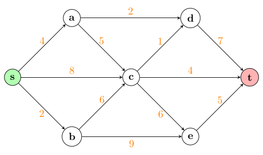
A network can be described as a directed graph , where is the set of nodes and is the set of arcs. Each arc has a capacity , which is the maximum amount of flow that can traverse the arc from node to node .
The network flow problem can be defined as follows: Given a network , a source node , a sink node , and capacities on the arcs, find the maximum flow from to that respects the capacity constraints.
For example, consider the directed graph here with capacities on the arcs.
Example 4.12: Airline Transfer Network: Maximizing Passenger Throughput
An airline is trying to reroute as many stranded passengers as possible from an origin city () to a destination city () using a network of connecting flights. Each flight has a known number of available seats, and passengers may transfer at intermediate airports. The objective is to determine the maximum number of passengers that can be routed from origin to destination, using available seat capacity and respecting flight routes.
The network includes:
Origin airport ,
Intermediate hubs: ,
Regional transfer airports: ,
Final destination airport ,
Directed flight legs (arcs) with known seat availability.
Sets and Parameters:
: set of airports.
: set of flight legs.
: number of available seats on flight from airport to for all .
Variables:
:
number of passengers assigned to fly from airport to for all
Model:
In compact summation notation form, we have
This model helps the airline determine how to assign passengers to flight legs in a way that makes maximum use of the network’s available capacity. It is especially useful during disruption scenarios like:
severe weather cancellations,
emergency rerouting due to maintenance issues,
high-demand events requiring temporary overflow routing.
The same framework can be extended to include priorities, time windows, or rebooking costs.
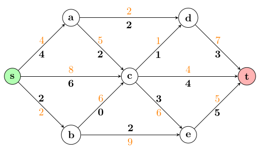
The solution is shown here in bold values on the graph. There is a total flow of 12.
The maximum flow problem can be written mathematically in the following
way.
Sets:
: Set of nodes in the network.
: Set of arcs in the network.
Parameters:
: Capacity of arc , which is the maximum amount of flow that can traverse the arc from node to node .
: Source node.
: Sink node.
Variables:
: Flow on arc .
Model: The network flow problem can be formulated as a linear programming problem as follows:
Objective: - The objective is to maximize the total flow from the source node to the sink node .
Constraints: - Flow Balance: The first set of constraints ensures that the flow into each node is equal to the flow out of the node, except for the source and sink nodes.
- Capacity Constraints: The second set of constraints ensures that the flow on each arc does not exceed its capacity.
We will discuss duality later. But duality is a concept that helps create bounds on a problem. For this particular problem, we can think of a dual as a cut in the graph - something that separates from . For example:
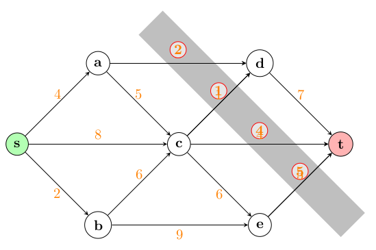
The selected arcs are a cut that separates from . The sum of their weights is , which implies that there is not a flow more than 12 units from to .
This bound is a form of duality. We will explore the concept more in later chapters. This duality is captured in the following theorem.
Theorem 4.13
The maximum flow amount is equal to the size of the minimum cut.
The multi-commodity minimum cost network flow problem is a generalization of the minimum cost network flow problem that considers multiple commodities flowing through the network. Each commodity has its own demand at each node and its own cost on each arc. The objective is to find the integer flow of minimum cost that satisfies the demands of all commodities at the nodes and the capacity constraints on the arcs.
A network can be described as a directed graph , where is the set of nodes and is the set of arcs. Each arc has a capacity . Each commodity has a demand at each node and a cost on each arc .
The multi-commodity minimum cost network flow problem can be defined as follows: Given a network , capacities on the arcs, demands and costs for each commodity , find the integer flow on the arcs for each commodity that minimizes the total cost of the flow, while satisfying the demands of all commodities at the nodes and the capacity constraints on the arcs.
Sets:
: Set of nodes in the network.
: Set of arcs in the network.
: Set of commodities.
Parameters:
: Capacity of arc .
: Cost per unit of flow of commodity on arc .
: Demand of commodity at node .
Variables:
: Flow of commodity on arc .
Model: The multi-commodity minimum cost network flow problem can be formulated as an integer linear programming problem as follows:
Objective: The objective is to minimize the total cost of the flow, summed over all commodities and all arcs.
Constraints:
Capacity Constraints: The first set of constraints ensures that the total flow on each arc (summed across all commodities) does not exceed its capacity.
Flow Conservation: The second set of constraints ensures that, for each commodity, the net flow into each node equals the demand of that commodity at the node.
Integrality Constraints: The third set of constraints ensures that the flow on each arc for each commodity is a non-negative integer.
Example 4.14: Multi-commodity network flow
[Excel] [PuLP] [Gurobipy]
Consider a small network with 4 nodes and 4 arcs, transporting 2 commodities. Each arc has a shared capacity, and each commodity has its own per-unit cost on each arc and its own supply/demand pattern at the nodes (negative values indicate supply, positive values indicate demand).
# Sample data
nodes = [1, 2, 3, 4]
arcs = [(1, 2), (1, 3), (2, 4), (3, 4)]
commodities = [1, 2]
capacities = {(1, 2): 20, (1, 3): 15, (2, 4): 25, (3, 4): 20}
costs = {(1, 2, 1): 2, (1, 2, 2): 3, (1, 3, 1): 3,
         (1, 3, 2): 2, (2, 4, 1): 1, (2, 4, 2): 2,
         (3, 4, 1): 2, (3, 4, 2): 1}
demands = {(1, 1): -10, (1, 2): -5, (2, 1): 0, (2, 2): 0,
           (3, 1): 0,   (3, 2): 0,  (4, 1): 10, (4, 2): 5}
The two figures below show the input network (left) and the optimal flow assignment (right). Each arc is labelled with the commodity flows it carries; the arc capacity constraint requires the sum of those commodity flows to stay within the arc’s capacity.
A common alternative formulation of the multi-commodity flow problem expresses each commodity in terms of a single source node, a single sink node, and a demand value, with flow variables that represent the fraction of the demand routed on each arc. The formulation below follows the description on the Wikipedia article https://en.wikipedia.org/wiki/Multi-commodity_flow_problem.
Problem Definition Given a flow network , where each edge has capacity , suppose there are commodities , defined by , where and are the source and sink of commodity , and is its demand. The variable denotes the fraction of commodity routed along edge ; we take when flow may be split among multiple paths, and when each commodity must follow a single path (“single path routing”). The problem is to find an assignment of all flow variables that satisfies the following four conditions.
(1) Link capacity. The total flow routed over any link, weighted by demands, does not exceed the link’s capacity:
(2) Flow conservation on transit nodes. For any intermediate node (other than the source or sink of commodity ), the flow of commodity entering equals the flow leaving :
(3) Flow conservation at the source. The full unit of commodity must leave its source:
(4) Flow conservation at the destination. The full unit of commodity must arrive at its sink:
Corresponding optimization problems. Three natural objective functions can be paired with the constraints above:
Load balancing minimizes the variation in link utilization ; a common linearization is to minimize the maximum utilization subject to for every arc.
Minimum cost multi-commodity flow attaches a per-unit cost to each arc and minimizes .
Maximum multi-commodity flow leaves the demands variable and maximizes the total throughput .
Relation to other problems. The minimum-cost variant generalizes the (single-commodity) minimum cost flow problem of Section 4.4.3 (which has only one source and one sink ). More broadly, every flow problem can be cast as a special case of the circulation problem.
Example 4.15: Source–Sink Multicommodity Flow
[Excel] [PuLP] [Gurobipy]
Consider the directed network on nodes with the arc capacities and per-unit costs listed below. Two commodities must be routed from source node to sink node : commodity 1 with demand and commodity 2 with demand .
| Arc | Capacity | Cost |
| 10 | 1 | |
| 8 | 2 | |
| 4 | 1 | |
| 7 | 3 | |
| 9 | 1 | |
Using the fractional flow variables with the minimum-cost objective and constraints (1)–(4), the optimal routing sends all of commodity 2 along and splits commodity 1 across the and paths (routing a small share through arc ), for a minimum total cost of .
The transportation problem involves determining the optimal way to transport goods from a set of suppliers to a set of markets. The goal is to minimize total transportation costs while satisfying supply availabilities at the suppliers and demand requirements at the markets.
Additional resources:
Let be the set of suppliers and be the set of markets.
Parameters:
: supply available at supplier
: demand required at market
: cost of shipping one unit from supplier to market
Variables:
: units shipped from supplier to market
Model:
The objective minimizes total shipping cost; the constraints ensure that the shipment from each supplier does not exceed its available supply, and that the demand at each market is satisfied. The decision variables specify the optimal shipment quantities.
This problem can be efficiently solved using specialized algorithms such as:
Successive Shortest Path Algorithm: Iteratively sends flow along the shortest-cost paths.
Cycle-Canceling Algorithm: Identifies negative-cost cycles and eliminates them to reach optimality.
Network Simplex Method: An adaptation of the simplex method designed specifically for network flow problems.
Linear Programming Solvers: General-purpose solvers such as the Simplex or Interior-Point methods can handle large instances.
Resources
Try it out visually!
Network Flow Problems: min-cost flow, transportation, and shortest path on interactive networks, with plain-language descriptions and applications.
Example 4.16: Multi-Period Capital Investment Problem
You are managing a multi-period investment fund with $50,000 to start. Over the course of four periods, you can allocate capital to a set of investment opportunities. Each investment requires an upfront cost and offers an expected payout at the beginning of the following period, which can then be reinvested. The goal is to maximize the total funds available at the end of the fourth period.
The following table lists the available investments, the required initial investment for each period, and their respective payouts for the next period. Formulate an LP to determine the optimal investment strategy over the four periods.
| Period | Investment | Investment Required ($) | Payout in Next Period ($) |
| 1 | A | 10,000 | 15,000 |
| 1 | B | 20,000 | 30,000 |
| 1 | C | 15,000 | 22,000 |
| 2 | D | 12,000 | 18,000 |
| 2 | E | 25,000 | 35,000 |
| 2 | F | 18,000 | 26,000 |
| 3 | G | 15,000 | 20,000 |
| 3 | H | 10,000 | 14,000 |
| 3 | I | 20,000 | 28,000 |
| 4 | J | 8,000 | 10,000 |
| 4 | K | 16,000 | 22,000 |
| 4 | L | 12,000 | 16,000 |
Solution
Variables:
: whether to invest
in opportunity
during period ,
where if
investment is
chosen in period ,
and
otherwise.
Parameters:
: investment required
for opportunity
in period .
: payout from
investment
in the next period.
Objective: The cash on hand at the end of period 4 is the payout of the period-4 investments:
Constraints:
Period 1 budget constraint:
Period 2 budget constraint:
Period 3 budget constraint:
Period 4 budget constraint:
Binary decision variables:
Case Study: Amazon Redraws Its Map: Regionalizing the Fulfillment Network
When you order from Amazon, the item might ship from a building 20 miles away or 2,000 miles away. Around 2023, Amazon restructured its US fulfillment network into largely self-sufficient regions so that most packages stay close to home: the “Regionalization” initiative. The redesign was driven by network optimization models, published in the INFORMS Journal on Applied Analytics, and made Amazon a 2025 Edelman Award finalist. In 2023 it reduced the cost to serve by $0.45 per item in the US while achieving Amazon’s fastest delivery speeds to date.
Serving a customer from a distant fulfillment center is expensive and slow, but keeping every product in every region requires more inventory. The network design must decide which connections (fulfillment center sortation delivery station) to operate and how demand should flow over them, balancing cost, speed, and capacity across thousands of facilities and arcs.
Model type: mixed-integer linear program on a network (with machine learning used only to forecast the inputs: demand, travel times). The published paper is explicit about this division of labor.
A simplified core of the “topology” model:
Sets and Parameters:
Let be the set of demand regions, with demand .
Let be the set of feasible fulfillment paths for region (a path uses specific facilities and transportation arcs); is the cost of serving one unit along path .
Let be the set of arcs with capacities .
Variables:
Let be the volume served on path .
Let if arc is operated (a connection Amazon chooses to run).
Model:
Note the second constraint: it is exactly the big-/linking trick from the integer programming chapter, with the capacity playing the role of . Regionalization shows up as the optimizer choosing to open mostly within-region connections.
Demands and travel times are forecasts, produced by machine learning models; the optimization treats them as data.
The deployed system also has a time-expanded “network timing” model producing hourly schedules; the topology model above is the strategic layer.
Deployed across Amazon’s US network in 2023: cost to serve fell by $0.45 per item, delivery speeds hit record levels, and the share of shipments fulfilled within their own region rose sharply.
“Regionalize and Scale: Amazon’s Fulfillment Network Design for Faster and Cheaper Delivery.” INFORMS Journal on Applied Analytics, 2025. https://doi.org/10.1287/inte.2025.0295
Exercise 4.17: Production Planning over Five Periods
This exercise mirrors Example 4.2 (Production Planning with 10 Periods) with a shorter horizon and new data. A plant must meet demand over periods. Production costs are dollars per unit in periods 1 through 5, demand is units, the holding cost is dollars per unit per period, and the initial inventory is .
Exercise 4.18: Machine Assignment with New Costs
This exercise mirrors Example 4.4 (Machine Assignment). The same workshop faces a new set of four jobs with cost matrix
where row gives the costs for machine and column corresponds to job (machines and jobs numbered through ). Write the assignment model for this data and find a minimum-cost assignment. As a check, the optimal total cost is .
Exercise 4.19: Warehouse Shipping with New Data
This exercise mirrors Example 4.10 (Minimum-Cost Network Flow). Keep the same network, supplies ( at Warehouse 1 and at Warehouse 2), and route capacities (, , , ), but change the data: the per-unit costs are now , , , on routes , , , , and the demands are now units at Store 1 and units at Store 2.
Exercise 4.20: Fair Housing Assignment for 12 Families
A new apartment complex has been completed, and 12 families need to be assigned to 12 available apartments. Each family has ranked the apartments (1 = most preferred, 12 = least preferred).
Download the data for this problem here data.
[§4.2]
Exercise 4.21: Maximum Network Flow to a Single Node
A disaster relief effort is underway to transport supplies to a central distribution hub in a flooded region. The network consists of multiple warehouses (nodes) that currently have varying inventory levels of emergency supplies. Each transportation route (arc) between warehouses is serviced by a single truck with a limited carrying capacity. The goal is to determine the optimal transportation plan that maximizes the amount of supplies delivered to the central hub while respecting inventory constraints and truck capacities on each route.
Formulate a max-flow optimization problem for this scenario. Define your decision variables, objective function, and constraints explicitly. Assume that you do not want to leave any inventory at the distribution centers.
| Node | Type | Inventory (if applicable) | Connected To | Capacity |
| W1 | Warehouse | 200 | D1 | 100 |
| W2 | Warehouse | 300 | D1, D2 | 150, 70 |
| W3 | Warehouse | 150 | D2 | 120 |
| W4 | Warehouse | 250 | D3, D1 | 100, 120 |
| W5 | Warehouse | 180 | D3 | 90 |
| D1 | Distribution | N/A | Hub, D2 | 200, 80 |
| D2 | Distribution | N/A | Hub | 180 |
| D3 | Distribution | N/A | Hub | 160 |
| Hub | Central Hub | N/A | — | — |
[§4.4.5]
Exercise 4.22: Max Flow
Write out the explicit constraints that define the max flow problem given in the picture. Solve this problem as a linear program using Excel.
[§4.4.5]
Exercise 4.23: Min Cost Network Flow
Use the picture below to formulate the corresponding capacitated min cost network flow. Each arc is labeled with its capacity (black) and its per-unit cost (red); the blue number at each node is its net demand (positive = demand, negative = supply). Solve this problem using Excel. As a check, the minimum cost is .
[§4.4.3]
Exercise 4.24: Transshipment Through Regional Hubs
Two factories ship a product to three stores through two regional hubs; no route connects a factory directly to a store. Factory A can supply up to units and factory B up to units. Stores , , require , , and units. The per-unit shipping costs are:
| A | 2 | 4 |
| B | 3 | 1 |
| 4 | 6 | 7 | |
| 5 | 3 | 2 | |
The hubs neither create nor store product: whatever enters a hub must leave it.
[§4.4.3]
Exercise 4.25: Assignment with Forbidden Pairs
Five workers must be assigned to five jobs, one job per worker and one worker per job. The cost matrix is
where rows are workers 1 through 5 and columns are jobs 1 through 5. Certification rules forbid worker 1 from doing job 2 and worker 4 from doing job 5.
Exercise 4.26: Multi-Period Inventory with a Production Cap
A plant can produce at most units per period. Over six periods, demand is units, production costs are dollars per unit, the holding cost is dollars per unit per period, and the initial inventory is .
[§4.1]
Exercise 4.27: Why Everything Ships Somewhere
Consider the minimum-cost network flow model of Section 4.4.3, with a flow-balance constraint at every node .
[§4.4.3]
Exercise 4.28: Integer Answers for Free
The assignment problem is stated with binary variables, but Section 4.2 notes that solving its LP relaxation (replace with ) still returns a binary assignment.
Exercise 4.29: Multicommodity Rerouting Under a Tighter Capacity
Return to the network of Example 4.14: nodes , arcs , , , with capacities , , , , commodity 1 sending units and commodity 2 sending units from node 1 to node 4, and the per-unit costs given in the example.
Exercise 4.30: Max-Min Fair Project Assignment
Three teams must each take on one of three projects. Team gives project a satisfaction score (higher is better):
The fairness discussion in Section 4.2 suggests maximizing the satisfaction of the worst-off team instead of the total.
[§4.2]
Solution
(Exercise 4.18) The model is the one in Example 4.4 with the new cost matrix: binary variables , one assignment constraint per machine and one per job, and objective . The optimal assignment is machine job (cost 3), machine job (cost 5), machine job (cost 2), and machine job (cost 3), for a total cost of . Checking all assignments confirms this is optimal; the next-best assignment costs .
Solution
(Exercise 4.21) Introduce one variable per transportation route: let be the number of units of supplies sent along the arc from node to node , for each arc in the picture (for example , , , and so on). The objective is to maximize the total amount reaching the hub,
There are three families of constraints. Each arc has a truck capacity, , where is the capacity written on the arc. Each distribution node passes along everything it receives, so flow is conserved there; for example at ,
and similarly at and . Finally, each warehouse can ship at most what it has on hand: the total flow leaving warehouse is at most its inventory. One caution about the “leave no inventory behind” request: writing the warehouse constraints as equalities makes the model infeasible, since for instance holds 200 units but its only outgoing route has capacity 100. So treat inventory as an upper bound on warehouse outflow and let the objective push as much through the network as the capacities allow.
Solution
(Exercise 4.22) Let denote the flow on arc . Maximize the flow arriving at subject to flow conservation at the four internal nodes and the arc capacities:
Solving this LP (in Excel or otherwise) gives a maximum flow of 19. One optimal flow is , , , , , , , , and all other arcs at 0. You can certify optimality without any theory: the two arcs into have capacities , so no flow can exceed 19, and this flow achieves it.
Solution
(Exercise 4.24) Introduce a flow variable for each of the ten arcs: from the factories to the hubs, and from each hub to each store. Supplies give and ; demands give for the three stores. The hub balance constraints are
Total demand () equals total supply, so both factories ship everything. An optimal plan sends , , , then , , , with minimum total cost
The structure is intuitive: factory B uses its cheap arc to , hub serves the stores it reaches cheaply ( and ), and store is served through .
Solution
(Exercise 4.30) For part 1, the assignment team project 1, team project 2, team project 3 has total satisfaction ; enumerating the six assignments shows this is the unique maximizer. For part 2, the same assignment gives minimum team satisfaction . A minimum of is impossible: team 1 scores at least only on project 1, while teams 2 and 3 score at least only on project 2, and both cannot have it. For part 3, the max-min LP achieves , for example with
which is doubly stochastic and gives every team an expected satisfaction of exactly . Fractions help because the max-min objective rewards evening out the teams: splitting projects lets the worst-off team trade some of another team’s surplus for its own shortfall. The total is linear, so in part 1 some optimal corner point is integral and fractions cannot improve it; the added constraints destroy that structure, exactly as in the two-team example of Section 4.2.


![The same four-node network annotated with a flow solution: arcs carry interval labels [5.0, 5.0] on 3 to 1, [10.0, 0.0] on 1 to 2, [10.0, 0.0] on 2 to 4, and [-0.0, 5.0] on 3 to 4, with boxed node labels [-10, -5], [0, 0], [0, 0], and [10, 5].](figs/modeling-sums-continued-tikz09.png)


