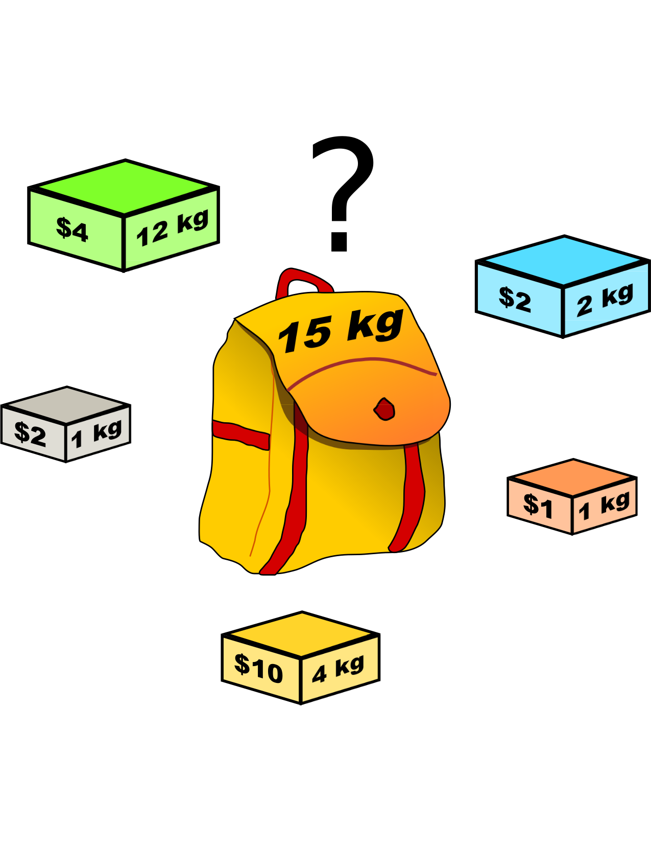
Image: See page for author [CC BY-SA 2.5].
https://en.wikipedia.org/wiki/Knapsack_problem
Learning Outcomes
Your linear program says to build 2.7 warehouses and route 3.4 trucks. Rounding up to 3 warehouses might blow the budget; rounding down to 2 might leave demand unmet; and neither rounded plan is necessarily anywhere near the best whole-number plan. Worse, many decisions are not quantities at all but choices (open this facility or don’t, assign this job to that machine or not) where “0.7 of a yes” means nothing. Requiring variables to take integer values looks like a small change to a linear program. It is not: it buys enormous modeling power, and this chapter is a tour of what that power can express.
In this section, we will describe classical integer programming formulations. These formulations may reflect a real world problem exactly, or may be part of the setup of a real world problem.
The knapsack problem can take different forms depending on if the variables are binary or integer. The binary version means that there is only one item of each item type that can be taken. This is typically illustrated as a backpack (knapsack) and some items to put into it (see Figure 15.1), but has applications in many contexts.
Image: See page for author [CC BY-SA 2.5].
https://en.wikipedia.org/wiki/Knapsack_problem
Binary Knapsack Problem
NP-complete
Given a non-negative weight vector , a capacity , and objective coefficients ,
| (15.1) |
Example 15.1: Knapsack
[Excel] [PuLP] [Gurobipy]
You have a knapsack (bag) that can only hold W = 15 kgs. There are 5 items that you
could possibly put into your knapsack. The items (weight, value) are given as: (12 kg,
4), (2 kg,
2), (1kg, 2), (1kg, 1), (4kg, 10).
Which items should you take to maximize your value in the knapsack? See
Figure 15.1.
Variables:
let if item is in the bag
let if item is not in the bag
Model:
In the integer case, we typically require the variables to be non-negative integers, hence we use the notation . This setting reflects the fact that instead of single individual items, you have item types of which you can take as many of each type as you like that meets the constraint.
Integer Knapsack Problem
NP-complete
Given a non-negative weight vector , a capacity , and objective coefficients ,
| (15.2) |
We can also consider an equality constrained version
Equality Constrained Integer Knapsack Problem
NP-hard
Given a non-negative weight vector , a capacity , and objective coefficients ,
Example 15.2: Min Coins
[Excel] [PuLP] [Gurobipy]
Using pennies, nickels, dimes, and quarters, how can you minimize the number of coins you need to make up a sum of ?
Variables:
Let be the number of pennies used
Let be the number of nickels used
Let be the number of dimes used
Let be the number of quarters used
Model:
The capital budgeting problem is a nice generalization of the knapsack problem. This problem has the same structure as the knapsack problem, except now it has multiple constraints. We will first describe the problem, give a general model, and then look at an explicit example.
Capital Budgeting
A firm has projects it could undertake to maximize revenue, but budget limitations require that not all can be completed.
Project expects to produce revenue dollars overall.
Project requires investment of dollars in time period for .
The capital available to spend in time period is .
Which projects should the firm invest in to maximize its expected return while satisfying its weekly budget constraints?
We will first provide a general formulation for this problem.
Capital Budgeting Model
Sets:
Let be the set of time periods.
Let be the set of possible investments.
Parameters:
is the expected revenue of investment for
is the available capital in time period for in
is the resources required for investment in time period , for in , for in .
Variables:
let if investment is chosen
let if investment is not chosen
Model:
Consider the example given in the following table.
| Project | [Revenue] | Resources required in week 1 | Resources required in week 2 |
| 1 | 10 | 3 | 4 |
| 2 | 8 | 1 | 2 |
| 3 | 6 | 2 | 1 |
| Resources available | 5 | 6 | |
Given this data, we can set up our problem explicitly as follows
Example 15.3: Capital Budgeting
[Excel] [PuLP] [Gurobipy]
Sets:
Let be the set of time periods.
Let be the set of possible investments.
Parameters:
is given in column “[Revenue]”.
is given in row “Resources available”.
is given in row , and column for week .
Variables:
let if investment is chosen
let if investment is not chosen
The explicit model is given by
Model:
The Capacitated Lot Sizing Problem (CLSP) is a fundamental optimization problem in production planning, where the goal is to determine an optimal production schedule that minimizes total costs while adhering to capacity constraints. The objective function accounts for production costs, setup costs, and inventory holding costs over a given planning horizon.
Let denote the number of discrete time periods, indexed by . The problem parameters are defined as follows:
is the demand in period ,
represents the unit production cost,
is the fixed setup cost incurred if production takes place,
denotes the unit inventory holding cost, and
represents the maximum production capacity in period .
The decision variables are:
denotes the quantity produced in period ,
is the inventory level at the end of period , and
is a binary variable that takes value 1 if production occurs in period , and 0 otherwise.
The CLSP can be formulated as the following mixed-integer linear program:
The objective function (Minimize total cost) minimizes the total cost over the planning horizon, incorporating production, setup, and inventory holding costs. The inventory balance constraint (Inventory balance) ensures that demand in each period is met using either inventory from the previous period or newly produced units. The constraint (Capacity and setup constraint) enforces production capacity limits and ensures that a setup cost is incurred when production occurs. Constraints (Non-negativity constraints) enforce non-negativity on production and inventory levels, while (Binary production decision) ensures that the setup decision is binary.
For simplicity, we assume an initial inventory level of zero.
The basic model of the facility location problem is to determine where to place your stores or facilities in order to be close to all of your customers and hence reduce the costs of transportation to your customers. Each customer is known to have a certain demand for a product, and each facility has a capacity on how much of that demand it can satisfy. We also need to consider the cost of building the facility in a given location.
This basic framework can be applied in many types of problems and there are a number of variants to this problem. Here we present the capacitated facility location problem. Additional variants and alternative formulations are covered in Book 2.
Capacitated Facility Location 1
NP-complete
Given connection costs , fixed building costs , demands , and facility capacities , the capacitated facility location problem is formulated as follows:
Sets:
Let be the set of facilities.
Let be the set of customers.
Parameters:
— the cost of opening facility .
— the cost of serving one unit of demand of customer from facility .
— the capacity (in units) of facility .
— the total demand (in units) of customer .
Variables:
— equals 1 if facility is opened; 0 otherwise.
— the number of units of customer ’s demand served by facility .
Model:
Example 15.4: Capacitated Facility Location: Retail Distribution Example
Context: A retail company plans to establish distribution centers across a country to serve its stores efficiently. The company faces decisions on which distribution centers to open and which stores each center should serve. Costs associated with opening each center and serving stores from them are known, and each center has a maximum capacity. Each store also has a known demand.
Given Data: (distribution-data.xlsx)
Number of potential distribution centers (): 3
Number of stores (): 4
Model Formulation: The capacitated facility location model described earlier can be applied to this scenario with the given data to determine the optimal number and location of distribution centers to open, and which stores each center should serve.
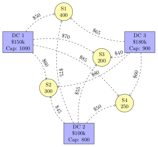
If you build and solve this instance, you will discover that it is infeasible: the stores demand units in total, while the three centers combined can supply at most . This is on purpose. Not every problem has a nice solution, and discovering infeasibility is itself useful information a model gives you. As an exercise, decide how you would repair the instance: reduce demand or add capacity.
Case Study: Where Should the Water Bombers Sleep? Airtanker Basing in Ontario
Ontario fights forest fires with a fleet of airtankers (water bombers). A fire caught within the first few hours is usually a small story; a fire missed grows into a big one. So the province’s ability to hit new fires quickly depends on where the airtankers are based each morning. In the early 1990s the Ontario Ministry of Natural Resources asked operations researchers to help decide the home bases, and the resulting mathematical programming model informed the province’s actual basing strategy from the 1993 fire season onward.
Fires do not announce where they will start. What is known is the historical pattern: some fire management zones see far more fire starts than others, and an airtanker can only provide effective initial attack on fires within a limited flying range of its base. With a fixed fleet, where should the aircraft be based so that as much expected fire activity as possible is within reach?
Model type: integer program (facility location / coverage). No machine learning; the fire-frequency inputs are historical averages.
Sets and Parameters:
Let be the set of fire management zones and the set of candidate bases.
Let be the expected number of fires in zone (from historical records).
Let if an airtanker based at can reach zone within the initial-attack time standard, and otherwise.
Let be the number of airtankers in the fleet.
Variables:
Let be the number of airtankers based at .
Let if zone is covered by at least one base within reach.
Model:
The version above counts a zone as covered or not; the published model is finer-grained, accounting for how many aircraft can respond and for daily fire-weather variation.
Expected fire counts stand in for actual (random) fire occurrence: the model optimizes the average day, not the worst day.
Airtankers can be re-deployed between bases day to day; the published work treats home-basing (seasonal) and daily deployment as linked decisions.
The Ontario Ministry of Natural Resources used the model to inform its airtanker home-basing strategy beginning with the 1993 fire season, and Ontario’s fire management program has continued to work with operations researchers for decades since, on deployment, dispatch, and detection-patrol planning.
J.I. MacLellan, D.L. Martell. “Basing Airtankers for Forest Fire Control in Ontario.” Operations Research 44(5), 677–686, 1996. https://doi.org/10.1287/opre.44.5.677
D.L. Martell. “The Development and Implementation of Forest Fire Management Decision Support Systems in Ontario, Canada.” Forest Ecology and Management / retrospective account, 2015.
D.L. Martell, R.J. Drysdale, G.E. Doan, D. Boychuk. “An Evaluation of Forest Fire Initial Attack Resources.” Interfaces 14(5), 20–32, 1984.
The set covering problem can be used for a wide array of problems. We will see several examples in this section.
Set Covering
NP-complete
Given a set with subsets , determine the smallest subset such that for all .
The set cover problem can be modeled as
| (15.6) |
where is a 0/1 variable that takes the value if we include item in set and if we do not include it in the set .
One specific type of set cover problem is the vertex cover problem.
Example: Vertex Cover
NP-complete
Given a graph of vertices and edges, we want to find a smallest size subset such that for every , either or is in .
We can write this as a mathematical program in the form:
| (15.7) |
Example 15.5: Set cover: Fire station placement
https://github.com/open-optimization/open-optimization-or-examples/blob/master/integer-programming/fire-station-covering.ipynb
In the fire station problem, we seek to choose locations for fire stations such that any district either contains a fire station, or neighbors a district that contains a fire station. Figure 15.3 depicts the set of districts and an example placement of locations of fire stations. How can we minimize the total number of fire stations that we need?
Sets:
Let be the set of districts ()
Let be the set of districts that neighbor district (e.g. ).
Variables:
let if district is chosen to have a fire station.
let otherwise.
Model:
Figure 15.4 shows how the neighborhood structure translates into a set cover instance, and Figure 15.5 gives an equivalent graph view of the same solution.
Set Covering - Matrix description
NP-complete
Given a non-negative matrix , a non-negative vector, and an objective vector , the set cover problem is
| (15.8) |
Example 15.6: Vertex Cover with matrix
An alternate way to solve equation is to define the incidence matrix of the graph. The incidence matrix is a matrix with entries. Each row corresponds to an edge and each column corresponds to a node . For an edge , the corresponding row has a in columns corresponding to the nodes and , and a 0 everywhere else. Hence, there are exactly two 1’s per row. Applying the formulation above in Graph representation of fire station problem. Every node is connected to a chosen node by an edge. models the problem.
We could also allow for a more general type of set covering where we have non-negative integer variables and a right hand side that has values other than .
Covering
NP-complete
Given a non-negative matrix , a non-negative vector , and an objective vector , the covering problem is
| (15.9) |
Case Study: Kidney Exchange: Integer Programming that Saves Lives
Thousands of kidney patients have a friend or family member willing to donate a kidney, but with the wrong blood or tissue type. Kidney exchange programs fix this with a swap: donor A gives to patient B while donor B gives to patient A. With three pairs, a three-way cycle works the same way. National programs, including the United States’ kidney paired donation program (UNOS) and the United Kingdom’s Living Kidney Sharing Scheme, decide who swaps with whom by solving an integer program. In the UK, that integer program runs on a fixed schedule several times a year: the solver’s output is literally the list of surgeries to schedule.
Given a pool of incompatible patient–donor pairs, find a set of swap cycles that gives as many patients as possible a compatible kidney. Two hard rules shape the problem. First, a pair can appear in at most one cycle (each donor has one kidney to give). Second, all surgeries in a cycle must happen simultaneously, so that no donor can back out after their loved one has received a kidney; operating-room logistics therefore cap cycles at two or three pairs.
Model type: pure binary integer program. No machine learning; compatibility is determined by medical testing.
Sets:
Let be the set of incompatible patient–donor pairs.
Let be the set of feasible swap cycles of length at most 3: subsets of pairs where each donor is compatible with the next patient around the cycle.
Variables:
Let if cycle is selected for surgery, and otherwise.
Model:
Here is the number of pairs in cycle , which equals the number of transplants the cycle produces. Real programs also include chains started by altruistic donors (someone who donates without a paired patient) and weight cycles by medical priority rather than just counting transplants; both are small extensions of the same model.
Compatibility is treated as a yes/no input from blood typing and tissue crossmatching, computed before the optimization.
The model shown maximizes the number of transplants; deployed programs maximize a weighted sum reflecting waiting time, sensitization, and pediatric status.
Enumerating all cycles is feasible for cycle length ; national-scale pools with long chains need column generation (a Book 2 topic).
Cycle- and chain-based integer programs are the clearing engines of the US and UK national programs, and the published models have been benchmarked directly on real UNOS and UK datasets. The UK scheme’s matching runs are performed with algorithms developed by the University of Glasgow. Economist Alvin Roth shared the 2012 Nobel Prize in part for the market design behind kidney exchange.
D.J. Abraham, A. Blum, T. Sandholm. “Clearing Algorithms for Barter Exchange Markets: Enabling Nationwide Kidney Exchanges.” Proceedings of ACM EC, 2007. https://doi.org/10.1145/1250910.1250954
D.F. Manlove, G. O’Malley. “Paired and Altruistic Kidney Donation in the UK: Algorithms and Experimentation.” ACM Journal of Experimental Algorithmics 19, 2015. https://doi.org/10.1145/2670129
R. Anderson, I. Ashlagi, D. Gamarnik, A.E. Roth. “Finding Long Chains in Kidney Exchange Using the Traveling Salesman Problem.” PNAS 112(3), 2015. https://doi.org/10.1073/pnas.1421853112
Graph coloring

Image: See page for author [Public domain], via Wikimedia Commons.
https://commons.wikimedia.org/wiki/File:Petersen_graph_3-coloring.svg
Figure 15.6is the problem of finding a minimum coloring in a graph, and it can be formulated in many ways. Each vertex is assigned a color and two vertices cannot share the same color if they are connected by an edge.
Since a graph on vertices never needs more than colors, we may fix the palette to be . For every vertex and every color in the palette, introduce a binary variable that equals exactly when vertex receives color . A second family of binaries records which colors actually get used: signals that color appears on at least one vertex. Minimizing the number of colors used then gives a classical integer programming formulation:
This basic model is highly symmetric: relabeling the colors in any feasible coloring produces a different solution with the same objective value, and a branch-and-bound solver may waste effort exploring all of these copies. We present two strengthened formulations from [?] that attack this symmetry; their paper goes further, adding several families of cutting planes.
Color order model: A coloring that uses colors can be encoded in many interchangeable ways—any labels chosen from will do. To keep a single representative from each such family, we force the labels to be consumed in numerical order: color is available only once color appears somewhere in the graph. Every coloring that skips a label, or that uses a label larger than the number of colors it needs, is thereby cut off. Two extra constraint families accomplish this:
The first ties to actual use of color ; the second forbids gaps in the label sequence. The number of feasible solutions drops dramatically.
Independent set order model: Even when labels are used in order, the color classes of a -coloring can still be shuffled among the labels , so symmetric copies remain. A more aggressive fix sorts the color classes by size: the vertices receiving color must be at least as numerous as those receiving color . This yields the constraints
which are more restrictive than those of the color order model.
As an exercise, try implementing these different models and compare the solve times.
In this section, we describe ways to model a variety of constraints that commonly appear in practice. The goal is changing constraints described in words to constraints defined by math.
Binary variables can allow you to model many types of constraints. We discuss here various logical constraints where we assume that for . We will take the meaning of the variable to be selecting an item.
| (15.10) |
| (15.11) |
Alternatively!
| (15.12) |
| (15.13) |
| (15.14) |
| (15.15) |
| (15.16) |
| (15.17) |
| (15.18) |
| (15.19) |
| (15.20) |
These tricks can be connected to create different function values.
Example 15.7: Variable takes one of three values
Suppose that the variable should take one of the three values . This can be modeled using three binary variables as
As a convenient addition, if we want to add the possibility that it takes the value , then we can model this as
We can also model variable increases at different amounts.
Example 15.8: Discount for buying more
Suppose you can choose to buy 1, 2, or 3 units of a product, each with a decreasing cost. The first unit is $10, the second is $5, and the third unit is $3.
Here, represents if we buy the th unit. The inequality constraints impose that if we buy unit , then we must buy all units with .
Big M comes again! It’s extremely useful when trying to activate constraints based on a binary variable.
For instance, if we don’t rent a bus, then we can have at most 3 passengers join us on our trip. Consider passengers and let be 1 if we take passenger and 0 otherwise. We can model the constraint that we can have at most 3 passengers as
We want to be able to activate this constraint in the event that we don’t rent a bus.
Let be 1 if we rent a bus, and 0 otherwise.
Then we want to say
If , then
We can formulate this using a big-M constraint as
| (15.21) |
Notice the two cases
In the second case, we choose to be so large that the second case inequality is vacuous. That said, choosing smaller values (that are still valid) will help the computer program solve the problem faster. In this case, it suffices to let .
We can speak about this technique more generally as
Big-M: If then
We aim to model the relationship
| (15.22) |
By letting be an upper bound on the quantity , we can model this condition as
| (15.23) |
Below are several applications of this modeling technique:
Facility Location with Fixed Costs:
To ensure that a facility
must be open in order to serve customer ,
we write
where is the quantity shipped and if facility is open.
Power Plant Operation Constraints:
A generator can only produce power when it is turned on. Letting
indicate that the generator is on at time ,
we write:
Task Scheduling with Precedence Constraints:
To ensure task starts
only after task
ends, if a binary
indicates the precedence relation is active, we write:
Routing and Time Windows:
In vehicle routing problems, to model time consistency across arcs, we use:
where indicates travel from node to node , and is service time at node .
Production Planning and Setup Costs:
To ensure production
is positive only if a setup decision
is made:
Example 15.9: Network Flow with Toll Charges Using Big-M Constraints
Consider a transportation network where some arcs incur a toll cost if used. Let:
be a directed graph with nodes and arcs .
be the flow on arc .
indicate whether arc is used.
be the per-unit flow cost on arc .
be the fixed toll incurred if arc is used.
be a large constant upper bound on possible flow through arc .
The objective is to route flow from a source node to a sink node at minimum total cost, including tolls when applicable:
Subject to:
Figure 15.7 illustrates a simplified transportation network over the five boroughs of New York City, with selected connections to model bridges and tunnels. Each node represents a borough, and directed arcs represent feasible travel routes. Some of these arcs include tolls, which are incurred only in one direction, mimicking real-world tolling policies.
Nodes. The nodes in the graph correspond to the following boroughs:
Manhattan
Brooklyn
Queens
Bronx
Staten Island
Arcs. The directed arcs model travel between boroughs, with an optional toll charge. These arcs represent crossings such as bridges or tunnels, and are defined as follows:
| From | To | Toll |
| Manhattan | Brooklyn | Yes (e.g., Brooklyn-Battery Tunnel) |
| Manhattan | Queens | Yes (e.g., Queens-Midtown Tunnel) |
| Brooklyn | Queens | No |
| Manhattan | Bronx | Yes (e.g., RFK/Triborough Bridge) |
| Bronx | Queens | Yes |
| Manhattan | Staten Island | Yes (e.g., Verrazzano-Narrows Bridge) |
| Staten Island | Brooklyn | No |
Toll Modeling. Each arc in the network has an associated binary toll flag. If a toll applies, the arc is subject to a fixed toll cost only if it is used. This can be modeled in a mixed-integer program using a binary variable that indicates whether the arc is selected. A Big- constraint of the form:
can be used to enforce toll cost and flow constraints, where is the flow over arc , and is a suitably large upper bound on the possible flow.
Legend. In the figure, solid green arrows represent toll-free travel, while dashed red arrows indicate that a toll is applied in the direction of the arc.
Case Study: 108, 000 Fewer Truck Routes: Walmart’s Load Planning
Walmart moves goods from distribution centers to about 4,700 US stores on one of the largest private trucking fleets in the world. For the 2023 Franz Edelman Award (which it won), Walmart described an end-to-end optimization framework, from long-term network design down to daily routing and trailer load planning. In fiscal year 2023 the system eliminated 108,000 truck routes and 33 million driving miles, saving $91.5 million and preventing 98.6 million pounds of CO emissions.
Every day, each store needs a set of orders delivered. Orders take up trailer space; trucks have capacity; stores have delivery windows; and every truck dispatched costs money and emissions. The daily question at the heart of load planning: pack the orders into as few trailer-loads as possible while respecting capacities and delivery requirements.
Model type: integer programming for load consolidation and routing, inside a framework whose strategic layers are also optimization models. Forecasts feed the models as data.
The consolidation core, simplified:
Sets and Parameters:
Let be the set of orders for a delivery region, with sizes (trailer cube).
Let be the set of available trailer-loads (trucks), each with capacity .
Compatibility data: if order can ride on truck (same route corridor, feasible delivery window).
Variables:
Let if order is loaded on truck .
Let if truck is dispatched.
Model:
The capacity constraint again uses the big- linking pattern with . The deployed system couples this packing decision with routing (which stores share a route) and with strategic network design; the Edelman paper describes the full architecture.
Order sizes and delivery windows are data; in practice they come from demand forecasts.
The simplified model minimizes truck count; Walmart’s objective also prices miles, so consolidating onto fewer, fuller, shorter routes is what produced the 33-million-mile reduction.
Routing (the order in which a truck visits stores) is a separate, harder layer, in Book 2 territory; this box shows the consolidation layer.
Deployed across Walmart’s US supply chain: 108,000 routes and 33 million miles eliminated in FY2023, $91.5 million saved, 98.6 million pounds of CO avoided. 2023 INFORMS Franz Edelman Award winner.
“Optimizing Walmart’s Supply Chain from Strategy to Execution.” INFORMS Journal on Applied Analytics 54(1), 5–19, 2024. https://doi.org/10.1287/inte.2023.0093
The Big-M technique from the previous subsection activated a single constraint. A closely related situation is when we have two constraints and we need at least one of them to hold: an inclusive or. For example, a delivery might need to arrive either before a morning deadline or after an afternoon opening, or a budget must be satisfied in at least one of two currencies. The trick is to use one binary variable to decide which constraint is enforced, and a pair of Big-M constraints to relax whichever one is not selected.
Either Or
| (15.24) |
can be modeled as
| (15.25) |
where is an upper bound on and is an upper bound on .
If , then the first constraint becomes , and the second becomes , which is trivially satisfied if is large enough.
If , then the second constraint becomes , while the first is relaxed as .
Either way, at least one of the two original constraints is enforced; the binary variable simply selects which one.
We now apply this recipe to a small example.
Example 15.10: Buses or Cars
To shuttle students to the football game, we need either at least buses or at least cars.
Let be the number of buses we have and
let be the number of cars that we have.
We want to enforce that or . Writing these in the form used above, we need or . Since , we may take as an upper bound on and as an upper bound on . The recipe gives
| (15.26) |
which simplifies to and . If we must have at least buses; if we must have at least cars.
Choosing Big-M Values. The constants and should be chosen as valid upper bounds on the expressions and , respectively, over the feasible region. Overly large values may weaken the LP relaxation and cause numerical instability, so careful bounding is recommended whenever possible. In the example above, the bounds and are as tight as possible.
Use Cases. Either-or constraints naturally arise in problems with conditional decisions, such as:
If a machine is used, then either a certain energy constraint or a safety constraint must be met.
In facility planning, either a site must be built with one configuration or another.
In piecewise models where a variable must fall into one of two feasible regions.
We will see a substantial application of this idea, with more than two constraints in the disjunction, when we study 2D packing problems in Section 15.7.4.
Suppose that we want to model the fact that if we have at most 10 students attending this course, then we must switch to a smaller classroom.
Let be 1 if student is in the course or not. Let be 1 if we need to switch to a smaller classroom.
Thus, we want to model
If
then
Using the recipe below with , (the data are integer), and lower bound on , we can model this as
| (15.27) |
If , the constraint forces at least students; equivalently (by the contrapositive), whenever or fewer students attend, the model must set .
If inequality, then indicator
We let be a lower bound on the quantity and we let be a tiny number that is an error bound in verifying if an inequality is violated. If the data are integer and is an integer, then we can take .
Now
| (15.28) |
can be modeled as
| (15.29) |
Proof. We now justify the statement above.
A simple way to understand this constraint is to consider the contrapositive of the if then statement that we want to model. The contrapositive says that
| (15.30) |
To show the contrapositive, we set . Then the inequality becomes
Thus, the contrapositive holds.
If instead we wanted a direct proof:
Case 1: Suppose . Then , which implies that
Therefore
After rearranging
Since and , the only feasible choice is .
Case 2: Suppose . By the choice of , this implies , so the inequality holds with . Since also , it holds with as well. Thus both choices of are feasible, as they should be. □
Many other combinations of if then statements are summarized in the following table:
These two implications can be used to derive the following longer list of implications.
Lastly, if you insist on having exact correspondence, that is, “ if and only if ” you can simply include both constraints for “if , then ” and “if , then ”. Although many problems may be phrased in a way that suggests you need “if and only if”, it is often not necessary to use both constraints due to the objectives in the problem that naturally prevent one of these from happening.
For example, if we want to add a binary variable that means
If does not affect the rest of the optimization problem, then adding the constraint regarding is not necessary. Hence, typically, in this scenario, we only need to add the constraint .
A disjunction is a generalization of an “or” statement. Suppose that we have constraints
and we want to enforce at least of them. This can be accomplished linearly by introducing a new binary indicator variable for each of the disjunctive constraints :
If , then the
th ensures that at least of the constraints are active.
Suppose we have a collection of rectangles and a 2-dimensional strip with width and infinite height. Each rectangle has width and height and we want to pack the rectangles into the strip so that (15.31a) overall height is minimized, (15.31b) overall width is less than , and (15.31c) none of the rectangles overlap. See Figure 15.8 for an example: Figure 15.8a shows the rectangles to be packed, and Figure 15.8b shows a packing whose overall height we wish to minimize.
Let denote the position of the lower-left-hand corner of each rectangle . The overlapping constraint (15.31c) is the trickiest part. Consider a pair of rectangles and : rectangle is located entirely to the left of rectangle if has a value larger than . That is, if . On the other hand, if , then rectangle is located entirely above rectangle . If either of these constraints is satisfied then rectangles and do not overlap. We could also place above or to the right of . This gives four constraints that we need to satisfy at least one of. The model can be thought of as follows:
Constraint (15.31c) is a set of four disjunctive constraints. This can be expressed linearly by introducing a new binary indicator variable for each of the disjunctive constraints in (15.31c):
If , then the
th ensures that at least one of the constraints is active. An optimal solution to the example is given in Figure 15.9; it was found via GurobiPy.This problem is considered strongly NP-Hard.
The modeling tricks so far in this section were built by hand out of binary variables and Big-M constraints. Certain logical structures come up so often, however, that modern solvers accept them directly as special ordered sets (SOS). Declaring an SOS constraint tells the solver about the structure explicitly, which both simplifies the model you write and lets the solver use specialized branching rules.
Definition 15.11: Special Ordered Sets of Type 1 (SOS1)
A Special Ordered Set of type 1 (SOS1) constraint on a vector indicates that at most one element of the vector can be non-zero.
SOS1 constraints arise whenever a set of options is mutually exclusive: choosing one supplier out of several, operating a machine in one of several modes, or assigning a shipment to one of several routes. If each has an upper bound , we could model this ourselves by introducing a binary variable for each and writing together with . Declaring an SOS1 constraint achieves the same effect with a single line of code and no extra variables.
The following small example is deliberately simple: the point is not the optimization problem itself, but seeing both modeling styles side by side in code.
Example 15.12: SOS1 Constraints
Solve the following optimization problem:
Since only one variable may be nonzero, the best choice is to push the variable with the largest objective coefficient, , to its upper bound: the optimal solution is with value .
Definition 15.13: Special Ordered Sets of Type 2 (SOS2)
A Special Ordered Set of Type 2 (SOS2) constraint on a vector indicates that at most two elements of the vector can be non-zero AND the non-zero elements must appear consecutively.
At first glance this looks like a strange condition to single out, but it is exactly what is needed to model piecewise linear functions: a point on a piecewise linear curve lies on one segment, and can therefore be written as a weighted average of the two consecutive breakpoints at the ends of that segment. We develop that application in the next subsection; here we first get comfortable with the constraint itself.
The example below modifies the SOS1 example in only one way (two consecutive nonzeros are now allowed), so the two examples are easy to compare. As before, the accompanying code shows both a binary-variable formulation and the one-line SOS2 declaration.
Example 15.14: SOS2
Solve the following optimization problem:
The pairs of consecutive variables are , , and . Comparing the objective coefficients, the best pair is at , giving value . Note that the SOS1 solution alone would give only .
Example 15.15: Piecewise Linear Function
Consider the piecewise linear function given by
We will use integer programming to describe this function. We will fix and then the integer program will set the value to .
Example 15.16: Piecewise Linear Function Application
Consider the following optimization problem where the objective function includes the term , where is the piecewise linear function described in Piecewise linear functions with SOS2 constraint:
Given the piecewise linear function, we can model the whole problem explicitly as a mixed-integer linear program.
| (15.39) |
If the solver does not support SOS2 constraints directly, we can enforce the same condition with binary variables. The recipe for a piecewise linear function with breakpoints is:
Write down pairs of breakpoints and functions values .
Define a binary variable indicating if is in the interval .
Define multipliers such that is a combination of the ’s and therefore the output is a combination of the ’s.
Restrict that at most 2 ’s are non-zero and that those 2 are consecutive.
Here the binary variable selects segment : the constraint picks exactly one interval , and the constraints then force for every index outside . Only and can be nonzero, which is exactly the SOS2 condition.
When the constraints could be general, we will write to define general constraints. For instance, we could have or or many other possibilities.
Consider the problem
Having the minimum on the inside is inconvenient. To remove this, we just define a new variable and enforce that and then we maximize . Since we are maximizing , it will take the value of the smallest . Thus, we can recast the problem as
There are a number of scenarios where the constraints can be relaxed without sacrificing optimal solutions to your problem. In a similar vein to maximizing a minimum, if because of the objective we know that certain constraints will be tight at optimal solutions, we can relax the equality to an inequality. For example,
Since the objective pushes each upward, we can relax the equality to
At any optimal solution of the relaxed problem, each is as large as its constraint allows, so holds and the optimal solutions are unchanged. This trick is valid whenever the objective pressure forces the relaxed inequality to be tight at optimality. Note that the direction matters: relaxing to instead would let the grow without bound.
In many formulations we need to enforce the constraint where . Note that the inequality version is equivalent to the pair of linear constraints and requires no integer variables. However, the equality defines a non-convex set (the union of and ), and so it cannot be modeled with linear constraints alone.
To handle this, decompose into its positive and negative parts: write with . Then provided that and are not simultaneously positive. We enforce this complementarity condition using a binary variable and a sufficiently large constant (an upper bound on in the context of the problem):
When , constraint (15.41) forces , so . When , constraint (15.40) forces , so . In either case, as required.
The technique above extends naturally to model the exact -norm constraint , where is a vector of decision variables and is a given constant. Such constraints appear, for example, in portfolio optimization where a budget constraint requires that long and short positions sum to a fixed investment level.
We introduce variables and binary variables for each component :
The bound is used here because no individual can exceed when the total -norm equals .
Suppose we need to model exactly. The inequality version can be modeled simply as for all , and if the objective is minimizing , the optimizer will push down to the true maximum. However, when the equality is required as a general constraint, we need to ensure that also satisfies for some .
Introduce binary indicator variables where indicates that achieves the maximum. With a sufficiently large constant :
The first set of constraints ensures for all . For the index where , the second constraint becomes , forcing . Together with the first constraints, this gives .
Try it out visually!
Job-Shop Schedule (Gantt): this chapter’s scheduling problem, solved and animated.
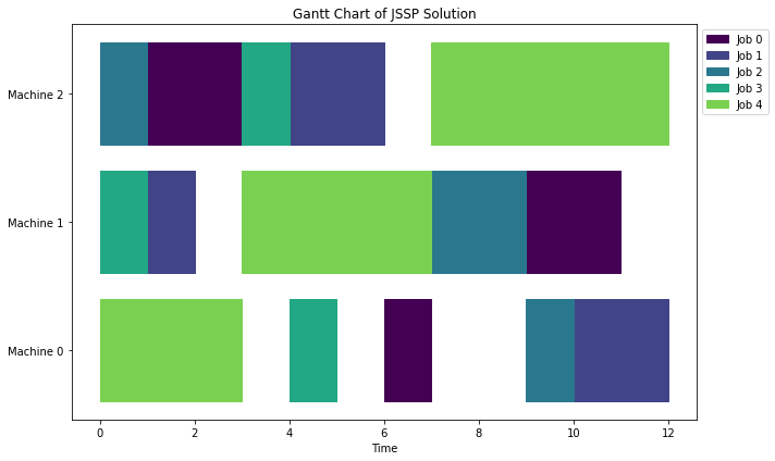
The Job Shop Scheduling Problem (JSSP) is a classical combinatorial optimization problem that is NP-hard. A set of jobs must be processed on a set of machines, where each job follows a prescribed sequence of operations across the machines. Each operation has a fixed processing time, each machine can handle only one job at a time, and once a machine begins processing an operation it must finish without interruption. The objective is to minimize the makespan, the time at which the last job completes.
Consider a small workshop with three machines (, , ) and four jobs. Each job must visit each machine exactly once, in a job-specific order, with the following processing times (in hours):
Job : .
Job : .
Job : .
Job : .
Processing jobs one after another (sequentially) yields a makespan of hours. By allowing jobs to run concurrently on different machines, the makespan can be significantly reduced.
Two pieces of data specify an instance. First, we collect the jobs in a set and the machines in a set . Second, each job carries its own route through the shop together with the time it needs at each stop: we write for the machine on which job runs its -th operation, so that the route of job is the sequence , and we write for the time job occupies machine .
A schedule assigns a start time to every operation. Three rules separate the feasible schedules from the infeasible ones: the operations of a job may not start out of order—each waits for its predecessor on the route to finish; a machine hosts at most one job at any moment; and processing cannot be paused, so an operation that starts at time on machine blocks that machine until time . Among all feasible schedules we want one whose makespan—the time when the final operation ends—is as small as possible.
Example 15.17: Job Shop Scheduling Problem Input Data
Basic Parameters. Consider jobs and machines, using the workshop data introduced above.
Processing Times. The matrix of processing times (one row per job, one column per machine) is:
The entry in row , column gives the processing time of job on machine .
Machine Sequences. The order in which each job visits the machines is:
Each row gives the machine sequence for a job. For instance, job 1 is processed first on machine 1, then machine 2, then machine 3, while job 3 starts on machine 3, then visits machine 1, and finishes on machine 2.
Big Calculation. A large constant is used in the big- formulation to enforce disjunctive constraints. A valid choice is the sum of all processing times:
Applications of JSSP The JSSP has numerous practical applications, including:
Manufacturing: Scheduling tasks in a production line to optimize throughput.
Computer Science: Allocating tasks to processors in parallel computing environments.
Healthcare: Scheduling surgeries and other treatments in hospitals.
Transportation: Optimizing maintenance tasks for vehicles or aircraft in a maintenance facility.
We now build a mixed-integer program from the ingredients above. This disjunctive formulation is classical and is due to Manne1.
Sets:
, the jobs.
, the machines.
Parameters:
, the machine hosting the -th operation of job ; row of the matrix from the example lists these machines in order.
, the processing time of job on machine .
, a big- constant; the total processing time is always a valid choice, as computed for the example above.
Variables: The main decisions are continuous start times
together with a variable for the makespan. Start times alone cannot express “one of these two jobs must wait for the other,” so for each machine and each pair of jobs we add a binary variable that records which job goes first:
Constraints: Precedence within a job. Each job must follow its route: operation of job cannot begin until operation has finished, that is,
One job at a time per machine. Fix a machine and two jobs . Feasibility demands that either job clears the machine before job arrives, , or the reverse, . This is precisely the either-or situation of Section 15.7.2, and applying that recipe with in the role of the selector variable yields the big- pair
When the first inequality forces job ahead of job while the second is switched off; when the roles swap.
Makespan. The makespan must sit above the completion time of every job’s last operation:
Model:
| (15.42a) |
Solving this model on the four-job, three-machine instance above gives an optimal makespan of hours—a substantial improvement over the hours needed to run the jobs one at a time.
Example 15.18: Duplo Scheduling
[Excel] [PuLP] [Gurobipy]
The Duplo in-class exercise is solved with Gurobi in the link.
The optimal value is 11.
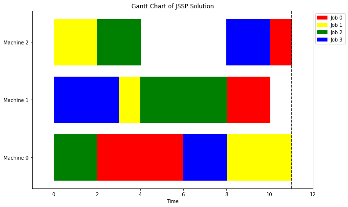

Makespan minimization of assigning jobs to machines.
In this variation, each machine can handle a number of different types of jobs. Some machines can do certain jobs faster than others.
We want to minimize the completion time of all of the jobs.
In this variation, each job visits its listed machines in sequence: most jobs require processing on two machines, in the order given, while a few need only one.
Machines:
Machine 1: Can perform jobs 1, 2, 3, 4, and 5
Machine 2: Can perform jobs 6, 7, 8, 9, and 10
Machine 3: Can perform jobs 11, 12, 13, 14, and 15
Machine 4: Can perform jobs 1, 6, 11, 2, and 7
Machine 5: Can perform jobs 3, 8, 13, 4, and 9
Jobs:
Job 1: Machine 1 (processing time = 2 hours), Machine 4 (processing time = 1 hour)
Job 2: Machine 1 (processing time = 3 hours), Machine 4 (processing time = 2 hours)
Job 3: Machine 1 (processing time = 2 hours), Machine 5 (processing time = 1 hour)
Job 4: Machine 1 (processing time = 4 hours), Machine 5 (processing time = 2 hours)
Job 5: Machine 1 (processing time = 1 hour)
Job 6: Machine 2 (processing time = 3 hours), Machine 4 (processing time = 2 hours)
Job 7: Machine 2 (processing time = 2 hours), Machine 4 (processing time = 1 hour)
Job 8: Machine 2 (processing time = 4 hours), Machine 5 (processing time = 2 hours)
Job 9: Machine 2 (processing time = 1 hour), Machine 5 (processing time = 1 hour)
Job 10: Machine 2 (processing time = 2 hours)
Job 11: Machine 3 (processing time = 3 hours), Machine 4 (processing time = 2 hours)
Job 12: Machine 3 (processing time = 2 hours), Machine 4 (processing time = 1 hour)
Job 13: Machine 3 (processing time = 4 hours), Machine 5 (processing time = 2 hours)
Job 14: Machine 3 (processing time = 1 hour), Machine 5 (processing time = 1 hour)
Job 15: Machine 3 (processing time = 2 hours)
Objective: Minimize the makespan (i.e. the total time it takes to complete all the jobs)
Constraints:
Each job can only be performed on the specified machines in the order listed
A machine can only work on one job at a time
There are no precedence constraints between jobs.
We leave this as an exercise for the reader to model and solve.
Exercise 15.19: Knapsack Problem
A hiker is packing a backpack with a weight capacity of 15 kg. The available items are:
| Item | Weight (kg) | Value |
| Tent | 5 | 8 |
| Sleeping Bag | 3 | 6 |
| Stove | 4 | 5 |
| Food | 7 | 10 |
| Camera | 2 | 4 |
Exercise 15.20: Courier Van Knapsack
A courier van can carry at most 15 kg on its last run of the day. Five packages are waiting, with weights and payouts:
| Package | 1 | 2 | 3 | 4 | 5 |
| Weight (kg) | 11 | 3 | 2 | 5 | 4 |
| Payout ($) | 5 | 3 | 3 | 7 | 4 |
[Example 15.1]
Exercise 15.21: Covering a Small Town
A town has six districts arranged in a grid:
| 1 | 2 | 3 |
| 4 | 5 | 6 |
Two districts are neighbors when their cells share a side. A fire station placed in a district covers that district and all of its neighbors.
Exercise 15.22: Big-M Activation Drill
A tour company runs three excursions with sign-up counts , where each excursion can take at most 30 tourists (). Let equal if the company hires a second guide. Company policy: if no second guide is hired, then the three excursions can take at most 40 tourists in total.
Exercise 15.23: Locating Distribution Terminals
Suppose that a company based in St. John’s is considering adding distribution
terminals in (1) Halifax, (2) Moncton, (3) Montréal, (4) Ottawa, and (5)
Toronto.
The cost of building the five terminals in millions of dollars would be 10 in Halifax, 12 in Moncton, 20 in Montréal, 18 in Ottawa, and 25 in Toronto.
Define the variables:
Using these variables, write a (binary) integer program that models the problem of determining which terminals to build subject to the constraints above that minimizes cost.
Exercise 15.24: Warehouse Location
A retail company must decide which of four potential warehouse sites to open. Each warehouse has a fixed opening cost and can serve a subset of five customer regions. The data are as follows:
| Warehouse | Fixed Cost ($1000s) | Regions Served |
| A | 150 | 1, 2, 3 |
| B | 200 | 2, 3, 4, 5 |
| C | 120 | 1, 4 |
| D | 180 | 3, 4, 5 |
Every customer region must be served by at least one open warehouse.
Exercise 15.25: Capital Budgeting with Dependencies
A firm is screening five projects over a two-year horizon. The net present values and the cash outlays (all in $1000s) are:
| Project | 1 | 2 | 3 | 4 | 5 |
| NPV | 20 | 40 | 20 | 15 | 30 |
| Year 1 outlay | 5 | 4 | 3 | 7 | 8 |
| Year 2 outlay | 1 | 7 | 9 | 4 | 6 |
The budget is 20 in each year. In addition: project 3 is an expansion of project 1, so it can only be undertaken if project 1 is; and projects 2 and 5 would serve the same market, so at most one of them may be chosen.
Exercise 15.26: Facility Location: Two Distribution Centers
A company can open distribution centers at two sites to serve three stores. Opening costs, capacities, per-unit serving costs, and demands are:
| ($) | (units) | Store 1 | Store 2 | Store 3 | |
| Center 1 | 80 | 40 | $2 | $3 | $1 |
| Center 2 | 60 | 25 | $4 | $1 | $2 |
| Demand | 10 | 12 | 15 | ||
[§15.4]
Exercise 15.27: Coloring a Five-Node Graph
Consider the graph on vertices with edges
a five-cycle together with the chord .
[§15.6]
Exercise 15.28: Either-Or Constraints
A company produces two products, and . Production of product 1 requires a special machine that can either run in mode A or mode B, but not both simultaneously. The constraints are:
Mode A:
Mode B:
Exactly one of these two constraints must hold (the machine operates in exactly one mode). The objective is to maximize with .
Introduce a binary variable and a big- parameter to formulate this either-or constraint as a mixed-integer program.
[§15.7.2]
Exercise 15.29: Fixed-Charge Production
A factory can produce a product in any quantity , but starting up production incurs a fixed cost of . The variable production cost is per unit, and each unit sells for . The factory has capacity to produce at most 200 units.
[§15.7.1]
Exercise 15.30: Why Rounding the Relaxation Fails
Return to the knapsack instance of Example 15.1 and replace by (the LP relaxation).
[Example 15.1, Example 15.2, §15]
Exercise 15.31: When is Big-M Too Big?
In Exercise 15.28, the value is perfectly valid: the resulting mixed-integer program has the same optimal solution as with .
[Choosing Big-M Values paragraph in §15.7.2, Exercise 15.28]
Exercise 15.32: Reading the Kidney Exchange Model
Consider the cycle-selection integer program in the kidney exchange case study.
[Kidney exchange case study in §15.5.1]
Exercise 15.33: Piecewise-Linear Production Cost
A plant can produce up to 30 tons of product, sold at $6 per ton. Production cost is piecewise linear in the quantity : the first 10 tons cost $5 per ton, the next 10 tons cost $3 per ton (a bulk discount on inputs), and the final 10 tons cost $8 per ton (overtime).
[§15.7.7, Example 15.15, Example 15.14]
Exercise 15.34: Two Jobs, Three Machines
Two jobs must each pass through machines in that order. Processing times are:
Each machine can process only one job at a time, and jobs cannot be interrupted.
Solution
(Exercise 15.20) With if package is loaded, the model is
The optimal load is packages with weight and payout . The heavy package 1 never pays: taking it leaves only 4kg of room, and the best it can then achieve is .
Solution
(Exercise 15.21) The neighbor sets (including the district itself, as in the fire station example) are , , , , , . One station cannot cover all six districts since no set has more than four elements. Two stations suffice: districts and cover , and so do districts and , and districts and . The optimal value is , and these three placements are the only optimal ones.
Solution
(Exercise 15.26) Total capacity is , so the instance is feasible; in fact center 1 alone has capacity , while center 2 alone () does not suffice. Solving the model, the optimum opens center 1 only and serves all three stores from it: cost . Opening both centers costs in fixed charges plus in best-case serving costs, a total of , so the cheaper center is not worth its $60 opening cost.
Solution
(Exercise 15.27) The chromatic number is . Lower bound: vertices , , are pairwise adjacent (a triangle), so they need three distinct colors. Upper bound: the coloring , , , , is proper, as can be checked edge by edge. Solving the integer program confirms .
Solution
(Exercise 15.28) Introduce , where selects mode A and selects mode B. Valid big- values can be read from the problem: relaxing each constraint by (any upper bound on the left-hand sides over reasonable production levels works). The formulation is
If , mode A’s constraint is enforced and mode B’s is relaxed; if , the roles are reversed.
Solution
(Exercise 15.29) Let be the production quantity and indicate whether production is started:
The linking constraint plays two roles: if it forces (no production without paying the startup cost), and if it enforces the capacity limit of units. Since producing at capacity earns , the optimal solution is , .
Try it out visually!
Branch-and-Bound Tree Explorer: how solvers actually solve the integer programs in this chapter; watch branching, bounding, and fathoming on small examples.
Concept Quiz: twenty quick self-check questions spanning the whole book.
Resources
The AIMMS modeling book has many great examples. It can be found here: AIMMS Modeling Book.
For many real world examples, see this book Case Studies in Operations Research Applications of Optimal Decision Making, edited by Murty, Katta G. Or find it here.
GUROBI modeling examples by Open Optimization that are linked in this book
Knapsack Problem
Set Cover
Video! - Michel Bierlaire (EPFL) explaining set covering problem
See AIMMS - Media Selection for an example of set covering applied to media selection.
Facility Location
Other examples
Notes from AIMMS modeling book.
Modeling Tricks
Further Topics


