Learning Outcomes
Understand what happens to the optimal solution as we slightly vary the parameters
Calculate the range of parameters where the optimal solution (or optimal basis) remains optimal.
Understand the change of objective function value as parameters are changed.
Try it out visually!
Sensitivity Analysis Walkthrough: shadow prices, allowable ranges, and reduced costs derived step by step.
Duality and Sensitivity Explorer: change the data and watch the optimal solution and shadow prices respond.
Your bakery’s production plan is set, and the profit works out to $23. Then the phone rings twice. A neighboring shop offers to rent you one more hour of oven time; a supplier offers a deal on extra flour. Should you take either offer, and what is the most you would pay? Sensitivity analysis answers before you spend a dime: the extra hour would raise your profit by exactly $1, while the extra flour is worth nothing to you at all: you already have three units you aren’t using.
Every resource in a linear program has a price tag like this, telling you what one more unit of it is worth to your bottom line, and every such price tag comes with an expiration: it is only valid until the data move far enough that the optimal plan itself changes. Solving a linear program answers one question about one set of numbers. In practice the numbers (objective coefficients, resource limits) are estimates: prices move, machines break, a supplier delivers more flour than promised. Sensitivity analysis asks how the optimal solution and the optimal value respond when the data change, and how far the data can move before the answer changes structurally. All of this, including both claims in the story above, can be read from the final simplex dictionary, which is why optimization software such as Excel Solver reports it alongside the solution.
We return to the linear program solved by dictionaries in Chapter 7 and by tableaus in Chapter 9,
so that every range we compute here can be checked against the dictionaries and tableaus computed there. After applying the simplex method, we obtain the following optimal dictionary:
The current basis is , with nonbasic variables .
The optimal solution is:
Before any algebra, build intuition by dragging the right-hand sides and the objective slope in the Desmos sensitivity explorer (backup interactive explorer) and watching when the optimal vertex jumps to a different corner of the feasible region.
Three kinds of data appear in a linear program: the objective coefficients , the right-hand sides , and the constraint matrix . Before computing exact ranges, it is worth understanding qualitatively how each one enters the final dictionary.
The objective row of the revised dictionary is
where the coefficients of , namely , are the reduced costs. A change in lands in one of two places. If is a basic variable, then sits inside , so it moves the constant term : the optimal value changes linearly in for as long as the basis stays optimal. If is a nonbasic variable, then appears only in its own reduced cost: the current solution and objective value do not move at all until the change is large enough to flip the sign of that reduced cost, at which point variable wants to enter the basis and the current dictionary is no longer optimal.
The basic solution is , so a change in moves the basic variables directly. Small changes rescale while keeping it nonnegative, and the objective value moves linearly along with it. A large enough change drives some basic variable negative: the dictionary becomes infeasible, and restoring feasibility requires a pivot to a different basis (or reveals that the problem has become infeasible altogether).
Geometrically, changing tilts the corresponding constraint, reshaping the feasible region. Algebraically, the effect depends on which column is touched. If column is nonbasic, then is untouched; only the reduced cost of variable changes, and the current solution survives unless that reduced cost changes sign. If column is basic, the change alters itself, and since the entire dictionary is built from , even a small change can move the basic solution, every reduced cost, and the optimal value all at once.
| Change | Basic solution | Objective value | Basis change when… |
| (objective) | unchanged | moves if basic | a reduced cost changes sign |
| (RHS) | always moves | moves linearly | a basic variable hits |
| (matrix) | moves if basic | via reduced costs | feasibility or optimality breaks |
In the remainder of the chapter we make these statements quantitative for the running example: for each parameter we compute the exact range of values over which the current basis remains optimal, and how moves inside that range. We treat the right-hand sides first, then the objective coefficients, then redo both computations in matrix notation.
In standard form, a linear program is written as . We perturb one entry of at a time, holding the objective coefficients and constraint matrix fixed, and answer three questions:
Each case follows the same three moves: perturb the standard form, adapt the final dictionary, and read off the range.
The second constraint (corresponding to slack variable ) originally has RHS value . We now perturb this to , where , and investigate the effect.
Perturbed Standard Form (RHS of Constraint 2)
To isolate the effect of , define a new variable:
Substituting into the system yields:
➤ Adapt the final dictionary. Since the structure of the problem remains the same in terms of the new variable , we can substitute into the final dictionary:
Only the row of is affected: .
➤ Read off the range. To remain optimal, the dictionary must still satisfy feasibility: all basic variables must remain nonnegative when . Only depends on , so:
Since is a slack variable, the objective value does not move at all inside this range. Beyond it, and the current dictionary becomes infeasible, triggering a new pivot in the simplex method.
The first constraint corresponds to slack variable , which is currently nonbasic and set to 0 in the optimal solution. Its original right-hand side is . We now perturb it to , where , and examine how this affects the dictionary.
Perturbed Standard Form (RHS of Constraint 1)
To isolate the effect of , define a new variable:
Substituting into the system yields:
So the perturbed system is equivalent to the original, but now expressed in terms of .
➤ Adapt the final dictionary. We substitute into the optimal dictionary:
➤ Read off the range. To ensure the basis remains feasible, set and check that the basic variables remain nonnegative:
Feasibility conditions:
Thus, all conditions are satisfied when:
Within this range, the objective value changes linearly as . Outside this range, one or more basic variables becomes negative, and the current solution becomes infeasible, prompting a new pivot in the simplex method.
The third constraint corresponds to slack variable , which is currently nonbasic and equal to 0 in the optimal solution. Its original right-hand side is . We now perturb it to , where , and examine how this affects the dictionary.
Perturbed Standard Form (RHS of Constraint 3)
To isolate the effect of , define a new variable:
Substituting into the system yields:
So the perturbed system returns to the original structure but in terms of .
➤ Adapt the final dictionary. Substitute into the optimal dictionary:
➤ Read off the range. Now test feasibility at the basic solution :
Feasibility requires:
Thus, the allowable range for is:
Within this range, the objective value changes linearly as . Outside this range, or , and the dictionary becomes infeasible.
Recipe: RHS Ranging in the Dictionary
➤ Perturb Replace by and absorb into the constraint’s slack variable: restores the original right-hand side.
➤ Substitute Rewrite the optimal dictionary in terms of ; only the constant column changes, each constant shifting by a multiple of .
➤ Impose feasibility Require every basic variable at ; each row gives one linear inequality in .
✔ Read the range Intersect the inequalities. Inside the range, changes linearly in ; at an endpoint a basic variable hits , and any further change triggers a pivot.
Remark. Shadow Prices The rate at which changes with is called the shadow price of constraint . For the binding constraints we found : an extra hour or an extra unit of sugar is worth exactly in objective value, as long as stays within its allowable range. For the non-binding flour constraint (), the objective did not move at all: its shadow price is . This settles both phone calls from the start of the chapter: pay up to $1 for the extra oven hour (and no more than $1 total for up to one extra hour, since the price expires at ), and politely decline the flour. Shadow prices are the central objects of the next chapter, where they reappear as the variables of the dual linear program (Chapter 11).
Learning Checkpoint 10.2.1
The optimal dictionary gives when . What is the shadow price of constraint 1, and over what range of is that price valid? What happens to the shadow price at ?
We now examine how changes to the objective function coefficients affect the optimality of the current basis. In the original problem, the objective is:
We now perturb these coefficients to:
where . Recall the final dictionary:
with basis and nonbasic variables . Unlike an RHS change, a cost change never threatens feasibility (the solution stays where it is), but it can destroy optimality by making a reduced cost positive.
➤ Adapt the final dictionary. Let . Since is basic, we express the extra term in terms of the nonbasic variables using the dictionary row for :
Adding to the original dictionary , we obtain:
➤ Read off the range. To maintain optimality, the reduced costs of nonbasic variables and must remain . Thus:
So the allowable range for is:
Within this range, the objective value changes linearly as .
➤ Adapt the final dictionary. Let . Since is also basic, the perturbed objective becomes:
Adding to the original dictionary , we obtain:
➤ Read off the range. To maintain optimality:
So the allowable range for is:
Within this range, the objective value changes linearly as .
| Perturbed coefficient | Allowed range | Effect on objective |
Outside these ranges, the reduced costs of nonbasic variables become positive, violating optimality. In such cases, the simplex method would require a new pivot.
Recipe: Objective-Coefficient Ranging in the Dictionary
➤ Perturb Replace by . If variable is nonbasic, only its own reduced cost shifts by ; skip to the last step.
➤ Substitute If variable is basic, express the extra term in terms of the nonbasic variables using the dictionary row for , and add it to the objective row.
➤ Impose optimality Require every reduced cost (for a maximization problem); each nonbasic variable gives one linear inequality in .
✔ Read the range Intersect the inequalities. Inside the range the solution does not move, and changes linearly if is basic (not at all if is nonbasic).
Learning Checkpoint 10.3.1
Changing the objective coefficient of a nonbasic variable never changes the current optimal solution, but changing it enough can still change the optimal basis. Reconcile these two statements.
The dictionary manipulations above can be organized with matrices, which is how software carries them out. Writing the running example in standard form,
Let the basic variables be , and the non-basic variables be . Then the dictionary can be written as:
where:
Thus, explicitly:
or equivalently
The basis matrix is
Remark. Recovering
Partitioning into basic variables and slack variables , we write:
Hence, since the slack columns came from the identity matrix in the original , we conclude:
We modify the right-hand side of the first constraint and analyze its impact on feasibility:
Step 1 — Update the basic solution. Using the inverse basis matrix , the basic solution is :
Step 2 — Impose feasibility. Ensuring that all basic variables remain non-negative:
Step 3 — Read the range.
is the feasible range for that preserves the optimal basis, matching the range found with the dictionary in Section 10.2.
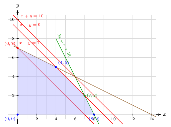
The figure below shows the constraint drawn for the three values .
To determine the range of values for (the coefficient of in the objective function) such that the current basis remains optimal, we analyze the simplex optimality conditions.
Step 1 — Set up the reduced costs. The objective function is initially:
The cost vector for all variables is:
The cost vector corresponding to the basic variables (i.e., the basis) is:
The reduced cost for any non-basic variable is given by:
The non-basic variables are and . We need to ensure that their reduced costs remain non-positive.
Step 2 — Compute the reduced costs for and . The constraint matrix is:
Extracting the columns corresponding to and :
Using the inverse basis matrix:
Thus, the reduced costs are:
Step 3 — Read the range. To retain optimality, we want and to be :
For the current basis to remain optimal, must satisfy:
matching the range found with the dictionary in Section 10.3.
When solving a problem in Excel, you can ask for a sensitivity analysis.
This will generate a report that will show the following:
Allowable Increase/Decrease: For each decision variable’s coefficient in the objective function, the report provides the range (allowable increase and allowable decrease) within which the coefficient can change without altering the current optimal basis. This range indicates the stability of the optimal solution with respect to changes in that coefficient.
Right-Hand Side (RHS) Values: For each constraint, the sensitivity report lists the shadow price (or dual value), which represents the rate of change in the objective function per unit increase in the RHS of that constraint. It also provides the allowable increase and allowable decrease for the RHS. These values indicate how robust the constraints are; small allowable changes might imply that the solution is sensitive to fluctuations in available resources or demand levels.
Constraint Status: The report shows which constraints are binding (active) and which are non-binding. A binding constraint has a positive shadow price and restricts the optimal solution, while a non-binding constraint has a shadow price of zero.
These are exactly the quantities computed by hand in Sections 10.2 and 10.3: the allowable increase/decrease columns are the ranges from the two recipe cards, and the shadow prices are the rates from the Shadow Prices remark.
For concreteness, the figures below show a worksheet set up for Solver and the sensitivity report it produces. Figure 10.3 shows the model layout — decision-variable cells, a SUMPRODUCT objective cell, and the constraint formulas — and Figure 10.4 shows the resulting report, with the allowable ranges, shadow prices, and binding status described above.
Exercise 10.1: Shadow Prices from the Final Dictionary
Recall the final dictionary of the running example of this chapter:
[§10.2]
Exercise 10.2: RHS Sensitivity Range
Consider the following linear program and its optimal dictionary:
The optimal dictionary is:
with basis and nonbasic variables .
Determine the range of values for (the RHS of the first constraint) for which the current basis remains optimal.
[§10.2]
Exercise 10.3: Objective Coefficient Sensitivity
Using the same linear program and optimal dictionary as in Exercise 10.2, determine the range of values for the objective coefficient (the coefficient of in the objective function) such that the current basis remains optimal. How does the optimal objective value change as varies within this range?
[§10.3]
Exercise 10.4: Full Sensitivity Workup
A shop assembles two products with profits $5 and $6 per unit:
Exercise 10.5: Ranging a Basic and a Nonbasic Coefficient
Consider the LP
whose optimal solution is with and basis .
Exercise 10.6: Sensitivity from the Basis Inverse
Consider the LP:
The optimal basis is with basis matrix and its inverse:
[§10.4]
Exercise 10.7: Reading a Sensitivity Report
The following is a sensitivity report from Excel Solver for a maximization LP with two decision variables and and three constraints:
| Variable | Value | Obj. Coeff. | Allow. Increase | Allow. Decrease |
| 8 | 6 | 2 | 3 | |
| 4 | 5 | 4 | 1 | |
| Constraint | Shadow Price | RHS | Allow. Increase | Allow. Decrease |
| 1 | 2.5 | 20 | 4 | 6 |
| 2 | 0 | 30 | 5 | |
| 3 | 1.0 | 12 | 3 | 2 |
[§10.5]
Exercise 10.8: Shadow Price Interpretation
A furniture workshop produces tables and chairs. The linear program is:
The optimal solution is , , with optimal profit . The dual solution is , .
[§10.2]
Exercise 10.9: Why a Slack Constraint Has Price Zero
Explain, in your own words, why a constraint that is not binding at the optimal solution must have shadow price . Give two arguments:
Exercise 10.10: Why Ranges Exist at All
Every quantity in a sensitivity report comes with an allowable range. Explain why.
Exercise 10.11: When the Shadow Price Prediction Breaks
Consider the LP
whose optimal solution is with . Note that all three constraints are tight there, but only two of them are needed to define the vertex: the optimal solution is degenerate.
Exercise 10.12: Pushing Past the Range
Construct a linear program with a constraint whose shadow price is some such that increasing the right-hand side of that constraint by increases the optimal value by exactly , but increasing it by increases the optimal value by strictly less than . Explain what happens at the boundary of the allowable range that makes the prediction fail, and verify your construction by solving the perturbed LPs. (Hint: the running example of this chapter already contains such a constraint.)
Solution
(Exercise 10.4)
so the shadow prices are : an assembly hour is worth $2 and a machine hour $1.
Solution
(Exercise 10.6)
so is a feasible basic solution with objective value .
Solution
(Exercise 10.8) At the optimal solution both constraints are binding: and .
Solution
(Exercise 10.12) The running example of this chapter works. Its hours constraint has shadow price , valid for (allowable increase ). Increasing by to raises the optimal value from to , exactly . Increasing by to raises it only to , not to : solving the LP with gives the optimum determined by the flour and sugar constraints, and . At the range boundary the basic variable hits and the basis changes; beyond it the hours constraint is no longer binding, so its shadow price drops to and further increases in buy nothing. In general, the optimal value is a piecewise-linear concave function of , and the shadow price is only its slope on the current piece.


