Learning Outcomes
Consider an introductory problem
Identify reasons for studying operations research
Define “Mathematical Programming”
Learn about different applications of the tools in this book
Explore the different types of optimization models and what types we will see in this book
Imagine you’re starting a new clothing company and decide to sell shirts. You’ve opened a store in Roanoke and, based on market research, you estimate the demand for the upcoming weekend:
Friday: 5 shirts
Saturday: 10 shirts
Sunday: 7 shirts
Your supplier can deliver shirts in one day, meaning an order placed on Thursday will arrive on Friday, and so on. As a business owner, you need to decide how many shirts to order and when to place each order to ensure you meet the daily demand without overstocking. Figure 1.1 shows the timing: each order arrives one day after it is placed, so Thursday’s order covers Friday’s customers.
Defining the Problem
To tackle this challenge, you’ll need to think strategically about two main factors:
Ordering Quantities: How many shirts to order on each day.
Inventory Levels: How many shirts to keep in stock at the end of each day.
You can define these decisions using variables:
Let the number of shirts you order on a specific day be a decision variable. For example, you could track the number of shirts ordered on Thursday, Friday, and Saturday.
Define variables to represent the number of shirts you have in stock at the end of each day.
Your goal is to meet the projected demand while managing costs. Costs could include:
The expense of ordering shirts.
The cost of holding inventory.
Penalties for running out of stock.
Refining the Scenario
As your business grows, additional complexities may arise. For instance:
The cost of ordering shirts might vary by day due to supplier pricing.
Holding inventory could incur storage costs.
A budget might limit how much you can spend on orders.
You might expand your product line to include pants and socks, each with its own demand and costs.
By clearly defining variables and constraints for these decisions, you can systematically approach the problem and develop an optimal strategy. This step-by-step process of defining the problem, incorporating real-world details, and refining the solution is a fundamental aspect of optimization.
This multi-stage example illustrates the iterative cycle of modeling:
Looking ahead, there are several ways to expand this scenario:
Expanding to New Stores: Opening additional stores introduces location-based demand, transportation costs, and coordination of inventory across multiple sites.
Hiring New Staff: Incorporate labor costs, scheduling constraints, and productivity rates into the model.
Producing Clothing In-House: Transitioning to manufacturing involves modeling production processes, including purchasing raw materials, machine capacities, and processing times.
Uncertain Demand: In reality, demand may be uncertain. Advanced models can incorporate stochastic elements or use probabilistic methods to handle randomness.
In this book, we will focus on deterministic models where all data is known and fixed. Building a strong foundation with these models will prepare us to tackle more complex problems involving uncertainty and randomness in future studies.
You already interact with optimization many times a day without noticing. The route your phone suggests, the price of your plane ticket, the fact that the store had what you wanted in stock, the schedule of your favorite sports league, and which kidney patients get matched with which donors: behind each one is an optimization model of the kind this book teaches. Even the AI assistants making headlines are trained by optimization; fitting a large language model is a nonlinear programming problem with billions of variables.
Operations Research (OR) is, in the words of the professional society INFORMS, a discipline that applies advanced analytical methods to help make better decisions. In a world where resources are limited and organizations face complex challenges, OR provides the tools and methodologies to model, analyze, and solve problems involving the optimal allocation of scarce resources. Studying OR equips individuals with a systematic and quantitative approach to decision-making, which is invaluable in industries such as logistics, finance, healthcare, and manufacturing.
By understanding OR, you gain the ability to construct mathematical models of real-world systems, allowing for the simulation and optimization of different scenarios. This leads to improved efficiency, reduced costs, and enhanced performance. The skills developed through studying OR, such as critical thinking, problem-solving, and data analysis, are highly transferable and sought after in today’s data-driven economy.
Operations Research also bridges the gap between theory and practice. It transforms abstract mathematical concepts into actionable strategies that can have a tangible impact on organizational success. Whether it’s optimizing supply chains, scheduling flights, or managing portfolios, the applications of OR are vast.
These are not hypothetical savings. A few documented examples:
Finalist projects for the INFORMS Franz Edelman Award, the field’s top prize for applied work, have documented cumulative benefits exceeding $446 billion since 1972 [?].
UPS’s ORION system optimizes delivery routes for tens of thousands of drivers; it cuts roughly 100 million miles of driving per year, worth $300–400 million annually, and about 100,000 metric tons of CO [?].
American Airlines’ yield-management system, an early large-scale optimization success, generated an estimated $1.4 billion over three years in the early 1990s [?].
Netherlands Railways rebuilt its national timetable with optimization, with a projected additional annual profit of about 40 million euros, and won the 2008 Edelman Award for it [?].
Every one of these is, at its mathematical center, the kind of model you will learn to build in this book.
Mathematical Programming is a core area within Operations Research that focuses on the formulation and solution of optimization problems. It involves creating mathematical models that represent the decision-making process of a system, where the goal is to find the best possible outcome under given constraints. The term “programming” in this context refers to planning or scheduling, not computer programming.
At the heart of Mathematical Programming is the objective function: a mathematical expression that defines the criterion to be optimized, such as minimizing costs or maximizing profits. The decision variables represent the choices available, and the constraints reflect the limitations or requirements of the problem, such as resource capacities or regulatory conditions.
There are various types of mathematical programming, each suited to different kinds of problems:
Linear Programming (LP): Deals with problems where both the objective function and constraints are linear.
Integer Programming (IP): Involves decision variables that must take on integer values.
Nonlinear Programming (NLP): Handles problems with nonlinear objective functions or constraints.
Dynamic Programming (DP): Breaks down problems into simpler subproblems and is particularly useful for multistage decision processes.
Mathematical Programming provides a powerful framework for optimizing complex systems and making informed decisions. It combines elements of mathematics, economics, and computer science to develop solutions that are both efficient and effective.
Operations Research and Mathematical Programming have a wide range of applications across various industries and sectors:
Transportation and Logistics: Optimizing routing and scheduling for delivery vehicles, reducing transportation costs, and improving supply chain efficiency.
Manufacturing: Streamlining production processes, managing inventory levels, and scheduling machinery to maximize productivity and minimize waste.
Finance: Portfolio optimization, risk assessment, and capital budgeting to enhance financial performance and manage uncertainties.
Healthcare: Allocating resources such as staff and equipment, scheduling surgeries, and managing patient flow to improve service quality and reduce wait times.
Energy Sector: Optimizing power generation and distribution, planning for renewable energy integration, and managing energy consumption.
Telecommunications: Network design and optimization, bandwidth allocation, and improving the reliability and efficiency of communication systems.
Agriculture: Planning crop rotations, optimizing the use of fertilizers and water, and managing supply chains for agricultural products.
Public Sector: Urban planning, emergency response logistics, and policy analysis to enhance public services and resource utilization.
Artificial Intelligence: Training machine learning models, including the large language models behind ChatGPT and Claude, by minimizing loss functions with nonlinear programming techniques.
Throughout the book, case-study boxes tell the stories of real deployed optimization models, each with the published model and its citation:
Preference-based housing assignment in Uruguayan cooperatives (assignment MIP), page 168.
The UN World Food Programme’s food baskets (diet LP + network MILP), page 85.
Amazon’s fulfillment-network regionalization (network design MIP), page 214.
Wildfire airtanker basing in Ontario (coverage location IP), page 867.
Kidney exchange in the US and UK national programs (cycle-selection IP), page 883.
Walmart’s truck load planning (packing IP; 2023 Edelman Award), page 910.
Each box states what kind of model was used, what was assumed, and where to read the original paper.
These applications demonstrate the versatility and impact of OR and Mathematical Programming. Using these tools, organizations can make data-driven decisions that lead to significant improvements in performance, cost savings, and competitive advantage. As global challenges become more complex, the importance of skilled professionals in Operations Research continues to grow.
We will state the main general problem classes to be associated with in these notes. These are Linear Programming (LP), Mixed-Integer Linear Programming (MILP), Non-Linear Programming (NLP), and Mixed-Integer Non-Linear Programming (MINLP).
Along with each problem class, we will associate a complexity class for the general version of the problem. Complexity classes are discussed in a later portion of the book. Although we will often state that input data for a problem comes from (as a real number), when we discuss complexity of such a problem, we actually mean that the data is rational, i.e., from (rational numbers that are encoded in the computer typically), and is given in binary encoding.
Warning
In the following subsections, we will use advanced notation that may be unfamiliar at this point. These mathematical notations will be developed throughout the book.
Also, don’t be too concerned about the specific definitions of the complexity classes at this point. For now, you can read that Polynomial time (P) means it should be relatively easy to solve, while the other classes might be much more difficult to solve.
Some linear programming background, theory, and examples will be provided in Part I of this book.
Linear Programming (LP)
Polynomial time (P)
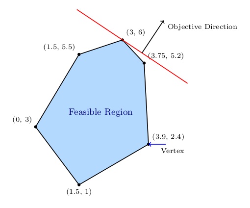
Given a matrix , vector and vector , the linear programming problem is
| (1.1) |
Linear programming can come in several forms, whether we are maximizing or minimizing, or if the constraints are or . One form commonly used is Standard Form given as
Linear Programming (LP) Standard Form
Polynomial time (P)
Given a matrix , vector and vector , the linear programming problem in standard form is
| (1.2) |
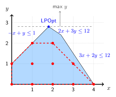
Mixed-integer linear programming will be introduced in chapter 15, with additional topics covered in Book 2. Recall that the notation means the set of integers and the set means the set of real numbers. The first problem of interest here is a binary integer program (BIP) where all variables are binary (either 0 or 1).
Binary Integer programming (BIP)
NP-complete
Given a matrix , vector and vector , the binary integer programming problem is
| (1.3) |
A slightly more general class is the class of Integer Linear Programs (ILP). Often this is referred to as Integer Program (IP), although this term could leave open the possibility of non-linear parts.
Integer Linear Programming (ILP)
NP-complete
Given a matrix , vector and vector , the integer linear programming problem is
| (1.4) |
An even more general class is Mixed-Integer Linear Programming (MILP). This is where we have integer variables and continuous variables . Succinctly, we can write this as , where stands for the cross-product between two spaces.
Below, the matrix now has columns, that is, . Also note that we have not explicitly enforced non-negativity on the variables. If there are non-negativity restrictions, this can be assumed to be a part of the inequality description .
Mixed-Integer Linear Programming (MILP)
NP-complete
Given a matrix , vector and vector , the mixed-integer linear programming problem is
| (1.5) |
NLP
NP-hard
Given a function and other functions for , the nonlinear programming problem is
| (1.6) |
Nonlinear programming can be separated into convex programming and non-convex programming. These two are very different beasts and it is important to distinguish between the two.
Here the functions are all convex!
Convex Programming
Polynomial time (P) (typically)
Given a convex function and convex functions for , the convex programming problem is
| (1.7) |
Observe that convex programming is a generalization of linear programming. This can be seen by letting and .
When the function or functions are non-convex, this becomes a non-convex nonlinear programming problem. There are a few complexity issues with this.
IP as NLP As seen above, quadratic constraints can be used to create a feasible region with discrete solutions. For example
has exactly two solutions: . Thus, quadratic constraints can be used to model binary constraints.
Binary Integer programming (BIP) as a NLP
NP-hard
Given a matrix , vector and vector , the binary integer programming problem is
| (1.8) |
Alternatively, consider the transformation where .
This can be reformulated with a single nonconvex constraint as
Machine learning is, at its mathematical center, learning functions from data. Instead of a person writing down the rule, we choose a family of functions with tunable parameters and let an optimization algorithm pick the parameters that fit the data best. The learned function might categorize data (is this email spam? does this scan show a tumor?), predict a number (tomorrow’s demand, a house price), or group similar things together without labels (customer segments, related news articles).
This is why machine learning belongs in an optimization book: training a model is solving an optimization problem, usually a continuous and often nonconvex one. The same recipe runs everywhere:
Spam filtering and fraud detection: classify a message or transaction as legitimate or not.
Demand forecasting: predict next month’s sales from history, weather, and promotions.
Image recognition: label the content of a photo, from unlocking your phone to reading medical scans.
Recommendations: predict which movie, song, or product a user will like next.
Large language models: systems like ChatGPT and Claude are trained by minimizing a loss function over billions of parameters, using nonlinear programming techniques (variants of gradient descent) run at enormous scale. The mathematics of training the most talked-about technology of the decade is the mathematics of this book’s nonlinear programming chapters.
Below are the two most common mathematical shapes these problems take. We will see both in greater detail later in the book.
In supervised learning, this objective is typically a loss function that quantifies the discrepancy between the predictions of a model and the true data labels. The aim is to adjust the parameters of the model to minimize this loss. Mathematically, this can be represented as:
| (1.9) |
where is the number of data points, is a per-data-point loss (e.g., squared error for regression or cross-entropy for classification), is the true label for the i-th data point, and is the model’s prediction for the i-th data point with parameters .
Clustering, on the other hand, learns structure with no labels at all: group the data so that points in the same group are similar and points in different groups are not. A retailer might cluster customers into segments for targeted offers; a biologist might cluster genes by expression pattern. One popular method is the k-means clustering algorithm. The objective of k-means is to partition the data into clusters by minimizing the within-cluster sum of squares (WCSS). The mathematical formulation can be given as:
| (1.10) |
where represents the j-th cluster and is the centroid of that cluster.
This encapsulation presents a glimpse into how ML problems are framed mathematically. In practice, numerous algorithms, constraints, and regularizations add complexity to these basic formulations.
MINLP
NP-hard
Mixed Integer Nonlinear Programming (MINLP) combines elements of integer programming and nonlinear programming. In MINLP, some or all of the decision variables are constrained to be integers, and the objective function or constraints are nonlinear. A general MINLP problem can be formulated as:
| (1.11) |
where is the objective function, and are constraint functions, is a vector of continuous variables, and is a vector of integer variables.
MINLP is particularly challenging due to the nonlinearity in the objective and/or constraints and the discrete nature of some decision variables. It finds applications in various fields such as industry for process optimization, computational geometry, and machine learning for hyperparameter tuning.
In the convex case, both the objective function and the constraints are convex functions. This subclass is easier to solve compared to its non-convex counterpart.
Convex MINLP
NP-hard, but Polynomial time (P) in fixed dimension (typically)
For a convex MINLP, the problem is defined as:
| (1.12) |
Convex MINLPs, while still challenging, are typically more tractable due to the properties of convexity, which allow for more efficient solution methods.
Non-convex MINLPs are significantly harder due to the presence of non-convex functions, which can lead to multiple local minima.
Non-Convex MINLP
NP-hard(in fact, undecidable)
The non-convex MINLP problem is formulated as:
| (1.13) |
Non-convex MINLPs pose significant computational challenges due to the possibility of multiple local optima and the inherent complexity of integer constraints. These problems are common in real-world applications where decisions are discrete, and the system behavior is non-linear and complex.
MINLP problems are known for their computational complexity, primarily due to the combination of non-linearity and integrality. The non-convex variants, in particular, are NP-hard, making them some of the most challenging problems in optimization.
In practice, MINLP models find extensive applications across various domains. In industry, they are used for complex decision-making processes like supply chain optimization and production planning. In computational geometry, MINLP techniques help in solving problems like optimal packing or layout design. In machine learning, MINLPs are used for tasks like feature selection and hyperparameter optimization where discrete choices and nonlinear relationships are involved.
The versatility of MINLP models, combined with their inherent complexity, makes them an important area of study in optimization.
A comprehensive list of optimization software organized by problem type (including free solvers, commercial solvers with academic licenses, and modeling interfaces) is provided in Appendix E.
Optimization problems often involve uncertainty in their parameters, whether due to measurement errors, variability in input data, or unpredictable future events. Addressing uncertainty is crucial for developing solutions that are effective in real-world settings. Two primary approaches to optimization under uncertainty are stochastic optimization and robust optimization.
Stochastic optimization deals with problems where some parameters are uncertain but can be described probabilistically. In this framework, the optimization process incorporates the expected values, variances, or other statistical characteristics of uncertain parameters. Solutions are often evaluated based on their performance over a distribution of possible scenarios.
For example, in supply chain management, uncertain demand can be modeled using probability distributions. A company may aim to minimize costs while ensuring a high service level under varying demand conditions. Similarly, in finance, portfolio optimization often accounts for uncertain future returns by maximizing expected returns while managing risk.
Robust optimization, on the other hand, focuses on creating solutions that perform well across the worst-case realizations of uncertainty. Rather than assuming a specific probability distribution, robust optimization works with uncertainty sets, which define the range of possible values that uncertain parameters can take. The goal is to find solutions that are feasible and effective for all possible scenarios within the uncertainty set.
Applications of robust optimization include power grid operations, where uncertainties in demand and renewable energy generation need to be managed, and scheduling problems, such as airline crew scheduling, where disruptions must be minimized under varying operational conditions.
Optimization under uncertainty has a wide array of applications across industries:
Healthcare: Designing vaccination strategies to minimize the spread of diseases while accounting for uncertain infection rates and patient behaviors.
Transportation: Managing traffic flow or public transit schedules under uncertain demand and travel times.
Energy: Planning renewable energy investments and operations under uncertain weather conditions and energy prices.
Manufacturing: Ensuring production schedules are resilient to supply chain disruptions and variability in raw material quality.
Addressing the complexity of uncertain data typically makes these problems much harder than their deterministic counterparts. While these methods are powerful and applicable to a wide range of real-world scenarios, we will not focus on optimization under uncertainty in this textbook.
Exercise 1.1: Classify It: Production Plan
A juice company decides how many liters of apple juice and orange juice to produce. Each liter of apple juice earns $2 and each liter of orange juice earns $3. Pressing capacity gives , bottling capacity gives , and both quantities are non-negative. The company maximizes earnings. Classify this model as LP, ILP/BIP, MILP, NLP, or MINLP. Point to the two features of the model (type of functions, type of variables) that justify your answer.
Exercise 1.2: Classify It: Choosing Projects
A city can fund any subset of five park projects. Project costs dollars and benefits residents, and the budget is dollars. Let if project is funded and otherwise, and consider
Classify this model as LP, ILP/BIP, MILP, NLP, or MINLP, and justify your answer. What changes about the classification if the city can also fund a fraction of a project?
Exercise 1.3: Classify It: Fitting a Line
Given data points , we choose slope and intercept to minimize
with unrestricted. Classify this model as LP, ILP/BIP, MILP, NLP, or MINLP, and justify your answer. Is the objective function linear in the decision variables and ?
Exercise 1.4: Classify It: Warehouses with Congestion
A retailer decides which of candidate warehouses to open () and how much product to route through each open warehouse. Handling cost at warehouse grows quadratically with volume, so the objective includes terms , and product can flow through warehouse only if . Classify this model as LP, ILP/BIP, MILP, NLP, or MINLP, and justify your answer by naming which ingredient rules out each simpler class.
Exercise 1.5: Shirt Store: Variables and One Constraint
Return to the shirt store of Section 1.1: demand is 5 shirts Friday, 10 Saturday, and 7 Sunday, orders arrive one day after they are placed, and the store starts Thursday with no shirts.
Exercise 1.6: Spot the Pieces: Food Truck
A food truck owner must decide how many tacos and how many burritos to prepare tomorrow. Each taco uses 0.1 kg of meat and each burrito uses 0.25 kg, and only 30 kg of meat will be available. Prep labor is limited to 10 hours. Tacos earn $2 profit and burritos $3.50. Without writing the full model, identify in words: the decision variables, the objective function, and each constraint. State the units of every quantity you name.
Exercise 1.7: Spot the Pieces: Tutoring Center
A tutoring center schedules tutors for next week. It may hire each of 12 tutors for a whole number of one-hour sessions, at most 8 sessions per tutor. The center needs at least 40 total sessions covered, and its weekly budget is $900; tutor charges dollars per session. The center wants maximum total sessions within budget. Identify the decision variables, objective, and constraints in words. Then explain which model class from Section 1.5 fits this problem and why it is not simply an LP.
Exercise 1.8: Half a Bus
A school district’s model says the optimal fleet is 12.5 buses. A shirt store’s model says the optimal order is 2361.4 shirts.
Exercise 1.9: Why “Programming”?
The word “programming” in mathematical programming predates modern software. Explain in one or two sentences what the term refers to in this subject, and why “linear programming” does not mean writing computer code in a linear fashion.
[§1.3]
Exercise 1.10: Reading a Success Story
Pick one of the documented successes in the box “What is optimization worth?” in Section 1.2 (UPS ORION, American Airlines yield management, or the Netherlands Railways timetable). For your chosen system, describe: (a) what the decision variables likely were, (b) what objective was likely optimized, and (c) one constraint the model must have respected. You do not need to be exactly right; the goal is to translate a news-style claim into model components.
Exercise 1.11: Shirt Store: The Full Model
Formulate the complete shirt-ordering problem of Section 1.1 as a linear program. Demand is 5 shirts Friday, 10 Saturday, and 7 Sunday. Orders placed Thursday, Friday, and Saturday arrive the next day and cost $8, $9, and $10 per shirt respectively. Every shirt still in the store at the end of Friday or Saturday incurs a $0.50 holding cost for that night. The store starts with no inventory, all demand must be met on time, and leftover shirts after Sunday are allowed but earn nothing.
Solution
(Exercise 1.2) This is a binary integer program (BIP): the objective and the budget constraint are linear, and every variable is restricted to . If fractions of projects may be funded, replace with ; all constraints are then linear over continuous variables and the model becomes an LP.
Solution
(Exercise 1.5) Let be the shirts ordered on Thursday, Friday, and Saturday, and let be the inventory at the end of Friday and Saturday. Thursday’s order is all the store has on Friday, so Friday’s balance is
The constraint (together with this balance equation) is what forbids a Friday stockout: it forces .
Solution
(Exercise 1.9) Here “programming” means planning or scheduling: a “program” was a plan of activities, as in a military logistics program or a concert program. Linear programming is the construction of an optimal plan using linear relationships, and the term was coined before computer programming was common.
Solution
(Exercise 1.11) Let be the orders placed Thursday, Friday, Saturday, and the end-of-day inventories. The LP is
Covering a Saturday shirt by ordering Thursday costs , cheaper than the $9 Friday order; covering a Sunday shirt from Thursday costs , cheaper than $9.50 (order Friday, hold one night) and $10 (order Saturday). So the optimal plan orders everything on Thursday: , , with , , and total cost . Integrality is not a concern in this instance: the demands are integers and the optimal LP solution is already integer, so the LP and integer models agree.


